
1. Introduction
The temperature of a semiconductor element is a crucial parameter. It affects the operational lifetime of the semiconductor element. It affects the values of its electrical parameters. The shape of the semiconductor element's characteristics depends on its temperature. The semiconductor element's mode of operation depends on its temperature. A semiconductor operating at a lower temperature is less prone to failure [1].
Based on the Arrhenius equation, reducing the junction temperature from 150 °C to 100 °C increases the lifetime of the semiconductor by approximately 13 times. Lowering the junction temperature from 150 °C to 70 °C increases the lifetime of the semiconductor by about 87 times. The calculations were performed for an activation energy of Ea = 0.7 eV [2].
A semiconductor element consists of a casing. The outer part of the casing is made of epoxy resin. Inside the epoxy mold compound, there is an encapsulated semiconductor chip. The semiconductor chip is commonly referred to in the literature as the die. The chip is mounted on a base plate made of tinned copper. The connection to the die is provided through the leads. Some of the leads are embedded in the epoxy mold compound. Other leads are connected to the base plate. The base plate and leads are connected to the die via thin bonding wires. The bonding wires are embedded in the epoxy mold compound. In the following section of this study, the temperature of the semiconductor element Tdie should be understood as the temperature of the chip itself. Semiconductor elements are widely used in industry [3], [4].
There are two methods for indirect measurement of die temperature. In one method, the package temperature is measured using a temperature sensor [5]. This method is hazardous. There is a risk that the sensor may come into contact with a metal part of the casing. The metal part of the casing may be live. There is also a risk that the sensor will come into contact with the heat sink. The heat sink can also carry voltage. The thermal resistance between the sensor and the package of the semiconductor element is unknown. These disadvantages can be avoided by using infrared thermographic measurement.
Scientific publications describe methods for indirect thermographic measurement of the semiconductor element temperatures [6]. This procedure consists of two stages. In the first stage, a thermographic measurement of the case temperature Tc is performed. In the second stage, the relationship between Tc and the junction temperature Tdie is determined. This can be achieved using the finite element method (FEM).
In this study, the uncertainty of a single measurement is considered. This limits the scope of the Type B uncertainty analysis.
The literature describes methods for determining Type B uncertainty in thermographic temperature measurements [7], [8], [9]. The authors note that few publications are addressing the determination of uncertainty in indirect thermographic measurements of semiconductor element temperature.
2. Methods and measurement system
A. Finite element method
For the purpose of this study, the C2M0280120D transistor in a TO-247 package was selected. It is characterized by a drain current of Id=10 A and a gate-source threshold voltage of Vgs(th)=2.8 V [10]. The internal and external dimensions of the C2M0280120D case are shown in Fig. 1.
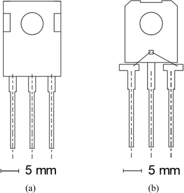
Fig. 1.
Package dimensions of the C2M0280120D transistor: (a) external dimensions and (b) internal dimensions (view after epoxy mold compound removal).
In the first stage of the research, it was necessary to obtain a reliable value of the transistor case temperature Tc. A dedicated measurement setup was constructed to achieve this. The main component of the setup was a Flir E50 thermographic camera operating in the long-wave infrared range. The long-wave infrared range is also referred to as long wavelength infrared (LWIR). The device uses an uncooled microbolometer detector array. The spatial resolution of the detector array is 180 × 240 pixels. The instantaneous field of view (IFOV) parameter is 1.82 mrad. This parameter enables accurate mapping of the transistor case surface corresponding to nine detector fields. The noise equivalent differential temperature (NEDT) value is 50 mK. This value ensures sufficient sensitivity for precise monitoring of surface temperature variations on the tested component [11].
The camera was mounted on a tripod. The distance between the camera and the tested object was d=33 mm. The entire measurement setup was placed inside a chamber made of transparent Plexiglas sheets. The chamber had dimensions of 40 × 30 × 30 cm. The interior of the chamber was lined with polyurethane foam. This lining minimized radiation reflections. The schematic of the constructed measurement setup is shown in Fig. 2.
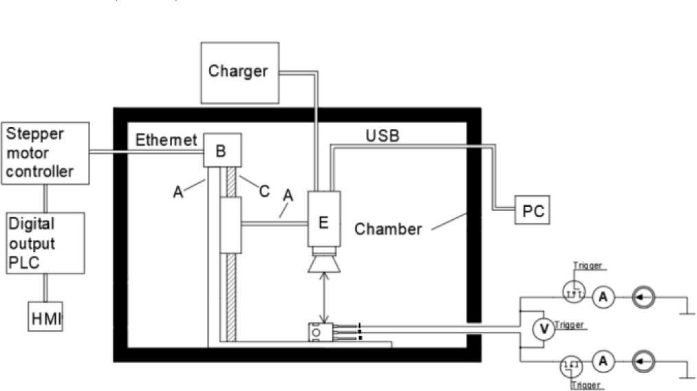
Fig. 2.
The diagram of the measurement circuit. A – the tripod, B – the stepper motor, C – the screw, E – the thermographic camera.
The second stage of the developed method involved determining the relationship between the temperatures Tc and Tdie. A three-dimensional relay model was created for this purpose. Creating this model required knowledge of the internal and external dimensions of the C2M0280120D case (Fig. 1). A cross-section of the case, together with the measured and determined quantities, is shown in Fig. 3.
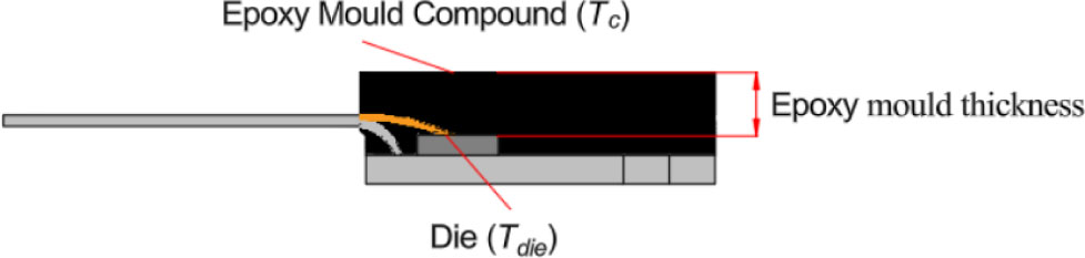
Fig. 3.
C2M0280120D package. Tc – thermographically measured temperature of the epoxy mold compound above the die. Tdie – temperature of the top surface of the die determined based on simulation studies.
The method FEM was applied. The simulations were carried out using SolidWorks software [12]. SolidWorks solves the heat conduction equation (1).
where:k – thermal conductivity [W·m−1·k−1],
ρ – density [kg·m−3],
ch – specific heat capacity [J/kg],
Q – heat sources [W· m−3],
T – temperature [K],
t – time [s].
For the discussed issues and under steady-state conditions, (2) can be used.
where:J – is a radiative heat flux [W·m−2],
x – direction.
After separating the variables, we integrated both sides of the equation, and evaluated the resulting time constant. Equation (2) can be rewritten in the form given by (3).
where:Pc – the total power, which was applied to the flat wall [W],
S – the area of the flat wall [m2], which was penetrated by J,
T1 – the temperature at the starting point of the analyzed heat flow path [K],
T2 – the temperature at the end point of the analyzed heat flow path [K],
xe – the end of the considered heat flow path (epoxy mold thickness) [m].
In order to perform the simulation studies (and to determine the relationship between temperatures Tc and Tdie), it is also necessary to determine the values of the radiation coefficient hr and the convection coefficient hc. The method for determining these values is described in detail in [6].
The finite element mesh of the created model is shown in Fig. 4(a). An example of the thermal simulation result for the created three-dimensional model is presented in Fig. 4(b). The location where the case temperature was measured is also shown in Fig. 4. The materials used in the developed model are presented in Table 1. The mesh element size and the corresponding simulation duration are presented in Table 2.
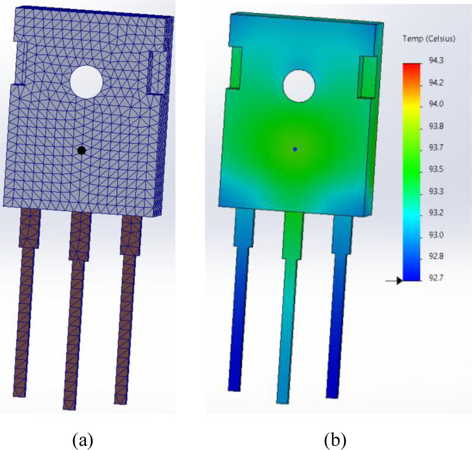
Fig. 4.
(a) The obtained model with the applied finite element mesh and the point at which the case temperature was measured, (b) simulation result of the C2M0280120D transistor obtained in SolidWorks, showing the resulting temperature distribution and the point at which the case temperature was measured (Tc value converted to °C).
Table 1.
The materials used in the developed model, along with their corresponding thermal conductivity coefficients k [13], [14], [15].
| Internal structure component | Material | k [W/m·K] |
|---|---|---|
| Black part of the case | EME 590 | 0.25 |
| Back part of the case | Copper | 400 |
| Semiconductor element | Silicon carbide | 150 |
| Lead, Internal connections | Copper | 400 |
| Grease | Melamine resin | 0.20 |
Table 2.
Mesh element size and the corresponding duration of the simulation.
| No. | Mesh element edge length [mm] | Simulation time [s] | ΔTcs [s] |
|---|---|---|---|
| 1 | 2.0 | 5 | 0.4 |
| 2 | 1.5 | 10 | 0.2 |
| 3 | 1.0 | 20 | 0.1 |
| 4 | 0.5 | 211 | 0.1 |
| 5 | 0.2 | 1455 | 0.1 |
Each simulation was performed 20 times. The chosen value minimized computation time while maintaining the stability of the results. The obtained data are summarized in Table 2.
B. Methodology of estimating uncertainty
To determine the Type B uncertainty, a measurement formula must be formulated. This can be done based on the radiative heat transfer model described in [11]. Subsequently, the Stefan–Boltzmann law should be applied. The method for deriving the measurement formula is described in detail in [16]. In this case (after taking into account the unsharpness), this equation takes the form of (4) [16], [17].
where:,
,
Wtot – the total radiation energy reaching the lens of the thermographic camera [W],
Ta – the ambient temperature [°C],
τa – the air transmittance [-],
Tl – the thermographic camera lens temperature [°C],
Trefl – the reflected temperature [°C],
ɛ – the emissivity [-],
τl – the lens transmittance [-],
Tus – the unsharpness temperature [°C].
The temperature difference between Tdie and Tc is described by (5).
where:Tdie – temperature of the top surface of the die determined based on simulation studies using the FEM [°C],
Tc – temperature of the C2M0280120D package measured using a thermal imaging camera [°C],
ΔpT – difference between Tdie and Tc.
To determine the uncertainty, the range of variability of the quantity xi from (4) was taken into account. Equation (6) was used for this purpose [18]. A rectangular probability distribution was assumed for all input quantities defined by variability ranges and lacking additional statistical information, in accordance with the Guide to the Expression of Uncertainty in Measurement (GUM). This assumption is justified by the lack of detailed statistical information and by the fact that only the limits of variability of the input quantities are known.
where:α – the half-width of the interval (semi-range).
A probability distribution is a function. This function defines the likelihood that a random variable takes on a specific value. This function also defines the likelihood that a random variable falls within a given range of values.
Afterward, the uncertainty contribution associated with the analyzed input quantity appearing in the measurement equation can be calculated. The measurement equation is given as (4). The uncertainty contribution is equal to the standard uncertainty of the analyzed input quantity multiplied by the sensitivity coefficient ci. The sensitivity coefficient ci describes how changes in the estimated value of the input quantity affect the estimated value of the output quantity. The value of this coefficient should be calculated separately for each input quantity. This can be done by calculating the derivative of the measurement function with respect to the given input quantity.
The standard uncertainty of Tc was determined using (7). It is denoted as u(Tc). It was obtained by calculating the square root of the sum of the squared uncertainty components ut(y). These components correspond to all terms appearing on the right-hand side of (4).
where:u(Tc) – the standard uncertainty of Tc,
xi – the ith input quantity in the measurement equation,
f – measurement function (4).
The expanded uncertainty U(Tc) is expressed in (8).
It was obtained by multiplying the combined standard uncertainty u(Tc) by the coverage factor k. Assuming an approximately normal distribution of the output quantity, justified by the Central Limit Theorem due to the combination of multiple input quantities with different probability distributions, a coverage factor k=2 was applied, corresponding to a confidence level of approximately 95 % [18].
Determining the value of measurement uncertainty using Monte Carlo simulations requires a different method. The document [19] sets a new standard for the calculation of measurement uncertainty. According to its interpretation, the measure of measurement uncertainty is the coverage interval. The coverage interval can be defined in two ways.
The first approach consists of determining a probabilistic symmetric interval. Outside this interval, the output quantity has an equal probability of occurrence. The second method states that it is the shortest permissible interval. These intervals are defined for the same coverage probability.
The determination of the expansion interval based on the first definition assumes equal probability of values on both sides of the interval. The coverage probability can be assumed to be 0.95. The interval limits are defined by the quantiles G−1(0.025) and G−1(0.975). These quantiles are the inverse functions of the cumulative distribution of the output quantity. Conventionally, this interval can be determined using (9).
The determination of the expansion interval based on the second definition requires selecting the smallest interval from the set of all possible intervals. These intervals correspond to the same probability. For a coverage probability of 0.95, this will be the interval whose upper and lower quantile limits yield the smallest difference. The quantile limits are G−1(α+0.95) and G−1(α). Conventionally, this interval can be expressed as (10).
where:Imin – minimum coverage interval of uncertainty,
G−1 – inverse cumulative distribution function (quantile function).
In this study, uncertainty was determined using the first approach. The first step was selecting the sampling number M. This number depends on the assumed coverage probability used to calculate the measurement uncertainty. For a coverage probability of p=95 %, this number was set to M=104. Next, sets of values for the input quantities were generated. These values were generated according to their assumed probability distributions. The same probability distributions for the input quantities were adopted as in the method based on the determination of measurement uncertainty using Type A and Type B approaches.
Subsequently, a set of possible output quantity values was determined. This determination was based on the measurement equation and the assumed input distributions. These values were arranged in ascending order. Consecutive probability levels were assigned to the values. The probability levels ranged from p=0.0001 to p=1. According to the first definition, the limits of the expanded uncertainty interval correspond to specific elements. These elements are number 250 and number 9750. A more detailed discussion of this approach can be found in publication [20].
3. Results
Using the measurement setup shown in Fig. 1, the difference between the thermal imaging camera readings ΔT was examined as a function of changes in the angle α of the thermal camera focus ring. The relationship between ΔT and the distance d was also investigated. The results are presented in Fig. 5 and Fig. 6.
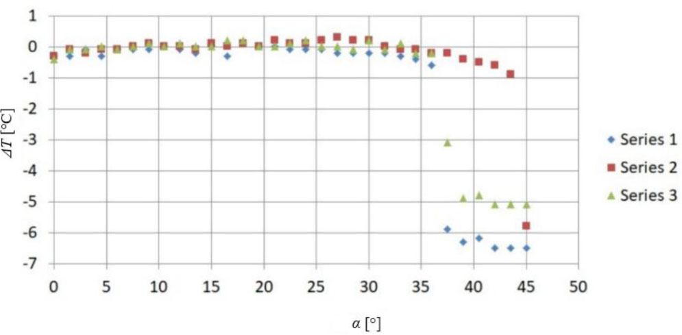
Fig. 5.
Relationship between ΔT and the angle α.
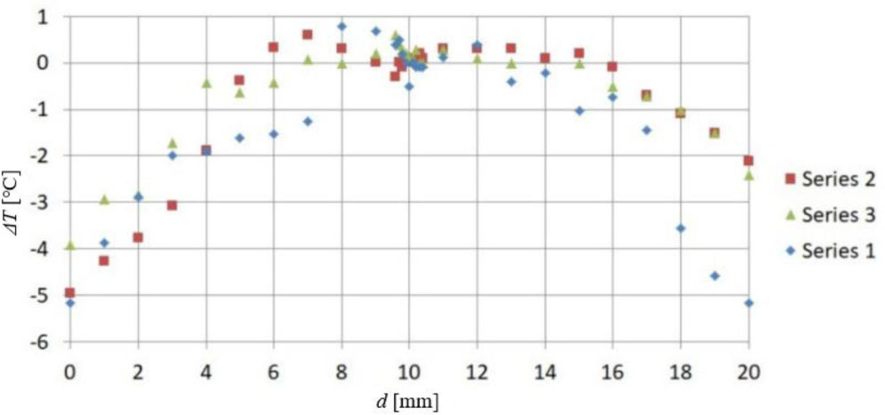
Fig. 6.
Relationship between ΔT and the distance d.
The results presented in Fig. 5 and Fig. 6 allowed evaluation of this effect. This effect concerns how much the thermographic temperature measurement uncertainty, determined without considering thermogram sharpness u(Tt) differs from that determined with thermogram sharpness u(Tt) taken into account.
Next, the range of variability of τa was examined. Publication [19] was used for this purpose. It was found that, under the conditions present during the experiment, the value of τa varied between 0.9 and 1. The emissivity ɛ was varied from 0.95 to 0.98. The reflected temperature Trefl ranged from 25 °C to 35 °C. The adopted value of τl corresponded to the transmittance of materials used in the construction of thermal imaging cameras operating in the LWIR range. The value of τl varied from 0.9 to 1.
An additional lens was installed on the thermal imaging camera. Therefore, it was assumed that Tl=Ta. As a consequence, the values of Tl were considered within the range of 18 °C to 35 °C. The final range of values was determined for Wtot. This quantity was calculated using (3). As a result, the highest Wtot value was determined to be 0.1669. The lowest Wtot value was determined to be 0.1439. The sensitivity coefficient ci was obtained as the partial derivatives of (4) with respect to all variables. The value of Tus was determined based on the analysis of the results presented in publication [16]. The value of Tus was also determined based on the results shown in Fig. 5 and Fig. 6. Additionally, this value was added to (4) as a correction term.
Analyzing the values in Table 3, it can be seen that Wtot and τl take the largest share of the determined uncertainty. This uncertainty is given in the last column of the table. The authors declare further work in this area. This work aims to reduce the values of these parameters. This reduction will lower u(x) and the final value of uncertainty.
Table 3.
Example uncertainty budget for an indirect thermographic measurement die with Tc=90 °C.
| Symbol xi | Unit | Estimate of quantity xi | Standard uncertainty u(xi) | Distribution of probability | Sensitivity coefficient c | Contribution of uncertainty ui(y) |
|---|---|---|---|---|---|---|
| τa | - | 0.9987 | 0.0010 | normal | 0.4488 | 0.0004 |
| Wtot | W/m2 | 0.1554 | 0.0066 | rectangular | 67.7701 | 0.4472 |
| ɛ | - | 0.97 | 0.0086 | rectangular | −7.6450 | −0.0657 |
| Trefl | °C | 30 | 2.8868 | rectangular | 0.0119 | 0.0344 |
| τl | m | 0.95 | 0.0289 | rectangular | −10.3189 | 0.2982 |
| Ta | °C | 26.5 | 4.9000 | rectangular | −0.0151 | −0.0740 |
| Tl | °C | 26.5 | 4.9000 | rectangular | −0.0151 | −0.0740 |
| Tus | °C | 3.25 | 1.88 | normal | 1 | 1.63 |
| Tc | °C | 90 | 3.25 |
As shown in Table 4, the value of the Type B uncertainty depends strongly on the value of the temperature Tc. An increase in the temperature Tc from 30 °C to 120 °C causes a more than threefold increase in the Type B uncertainty.
Table 4.
Type B uncertainty values for different temperatures Tc ranging from 30 °C to 120 °C.
| No. | Tc [°C] | u(Tc) [°C] |
|---|---|---|
| 1 | 30 | 1.63 |
| 2 | 60 | 2.44 |
| 3 | 90 | 3.25 |
| 4 | 105 | 4.21 |
| 5 | 120 | 5.17 |
To verify the correctness of the determined uncertainty budget, the uncertainty value was also calculated for the example shown in Table 3. In this case, the value of Tc was omitted. The obtained value was compared with the uncertainty value obtained using the Monte Carlo method. The results are presented in Table 5.
Table 5.
Standard uncertainty for the quantity Tc (package temperature).
| The value of the standard uncertainty | u(Tc) [°C] |
|---|---|
| Law of propagation of uncertainty | 1.63 |
| Monte Carlo method | 1.68 |
By comparing the results presented in Table 5, the values of the combined uncertainty uc obtained using both methods are very consistent. The relative difference between the two methods is approximately 3 %.
After verifying that the standard uncertainty u(Tc) obtained using both methods is comparable, the value of u(Tdie) was determined. A procedure similar to that used for determining u(Tc) was applied (6)–(9). In the constructed uncertainty budget, the value of ΔpT (5) was included by adding it to (4). The sensitivity coefficient ci for ΔpT was equal to 1. The remaining sensitivity coefficients c were selected in accordance with Table 3. The obtained results are presented in Table 6.
4. Conclusion
The standard uncertainty of thermographic temperature measurement is influenced by many factors. An analysis of the standard uncertainties and sensitivity coefficients for the individual components in the uncertainty budget presented in Table 3 reveals a significant contributing factor. This contributing factor to the overall uncertainty is the blurriness of the recorded thermogram.
This demonstrates an important requirement for thermographic temperature measurements of an electronic component performed using an additional Close-up 2× lens. Special attention must be paid to properly adjusting the sharpness of the recorded thermogram. Accurate compensation for the reflected temperature is also required. This is particularly important because the sharpness of the thermogram cannot be corrected after it has been recorded.
Some factors should be considered when creating an uncertainty budget for thermographic temperature measurement with an additional lens. These factors have only a marginal impact. They include ambient temperature and humidity. The change in the temperature value read from the thermogram due to its blurriness varies depending on the cause of the blurriness.
It should be noted that a thermogram becomes blurred when the distance between the lens and the observed object is incorrectly set. A thermogram also becomes blurred when the focus adjustment ring is improperly positioned. As a result, thermogram blurriness significantly affects the temperature value read from the thermogram. In such cases, the contribution of the factor related to variations in camera readings caused by increased thermogram blurriness will be substantial.
The contribution of this factor decreases when the sharpness of the recorded thermogram is improved. This demonstrates that the sharpness of the recorded thermogram must be properly adjusted to perform a thermographic temperature measurement of an electronic component with minimal error.
In this article, the results were obtained using Type B uncertainty evaluation. This evaluation was performed as described in the EA-4/02 guideline of European Accreditation. In future studies, these results should be compared with those obtained using other methods. One such method is the Monte Carlo approach.
Accurate determination of uncertainty requires knowledge of the types of distributions associated with the individual quantities in the uncertainty budget. This issue is closely related to the selection of an appropriate coverage factor. An incorrectly chosen coverage factor leads to an inaccurate estimation of the expanded uncertainty.
The values of measurement uncertainty were determined using the uncertainty propagation law method, as outlined in the Guide. The values were also determined using the Monte Carlo simulation method. The obtained values are very similar. This similarity confirms the usefulness of the Monte Carlo method for evaluating measurement uncertainty. Expanded uncertainty is commonly used as a measure of inaccuracy in metrology. It describes the symmetric dispersion of values for the measured quantity around its estimate.
The indirect thermographic measurement of a semi-conductor element's temperature is subject to uncertainty. As a result of the work carried out, the Type B uncertainty values were determined. These values take into account a number of influencing factors These quantities are presented in Table 3. The factor related to the blurriness of the thermogram Tus has a very significant influence on the Type B uncertainty value. The issue of the influence of blur on the thermographic temperature measurement of an electronic component's case is not widely described in the literature. It is described in document [21].
Nomenclature
- α
angle of the thermal imaging camera focus adjustment ring
- ɛ
emissivity of the surface of the tested element
- ρ
density
- σ
Stefan–Boltzmann constant
- τa
atmospheric (air) transmittance between the object and the camera
- τl
transmittance of the thermal imaging camera lens
- ΔT
temperature difference
- ΔpT
difference between Tdie and Tc
- α
the half-width of the interval (semi-range)
- ci
sensitivity coefficient of the output quantity with respect to the input quantity
- cf
specific heat
- d
distance between the camera lens and the tested object
- Ea
activation energy in the Arrhenius equation
- f
measurement function
- G−
inverse cumulative distribution function (quantile function)
- hc
convection coefficient
- hr
radiation coefficient
- IFOV
instantaneous field of view
- Id
drain current
- Imin
minimum coverage interval of uncertainty
- Isym
symmetric coverage interval of uncertainty
- J
radiative heat flux
- k
thermal conductivity
- ki
coverage factor
- M
number of samples in the Monte Carlo simulation
- NEDT
noise equivalent differential temperature
- Pc
the total power
- p
coverage probability
- S
the area of the flat wall
- Q
heat sources
- T
temperature
- T1
temperature at the starting point of the analyzed heat flow path
- T2
temperature at the end point of the analyzed heat flow path
- Ta
ambient temperature
- Tc
package temperature of the semiconductor lement (measured by a thermographic camera)
- Tdie
temperature of the semiconductor structure (determined based on simulation studies)
- Tl
temperature of the thermal imaging camera lens
- Trefl
reflected temperature of the tested object surface
- Tus
equivalent temperature error caused by thermogram unsharpness
- U(Tc)
expanded uncertainty of Tc
- u(Tc)
standard uncertainty of Tc
- U(Tdie)
expanded uncertainty of Tdie
- u(Tdie)
standard uncertainty of Tdie
- u(xi)
standard uncertainty of the i-th input quantity
- ut(y)
uncertainty components
- Vgs(th)
gate-source threshold voltage
- Wtot
total radiant energy density reaching the camera lens
- xi
i-th input quantity in the measurement equation
- xe
the end of the considered heat flow path
- y
output quantity of the measurement equation