
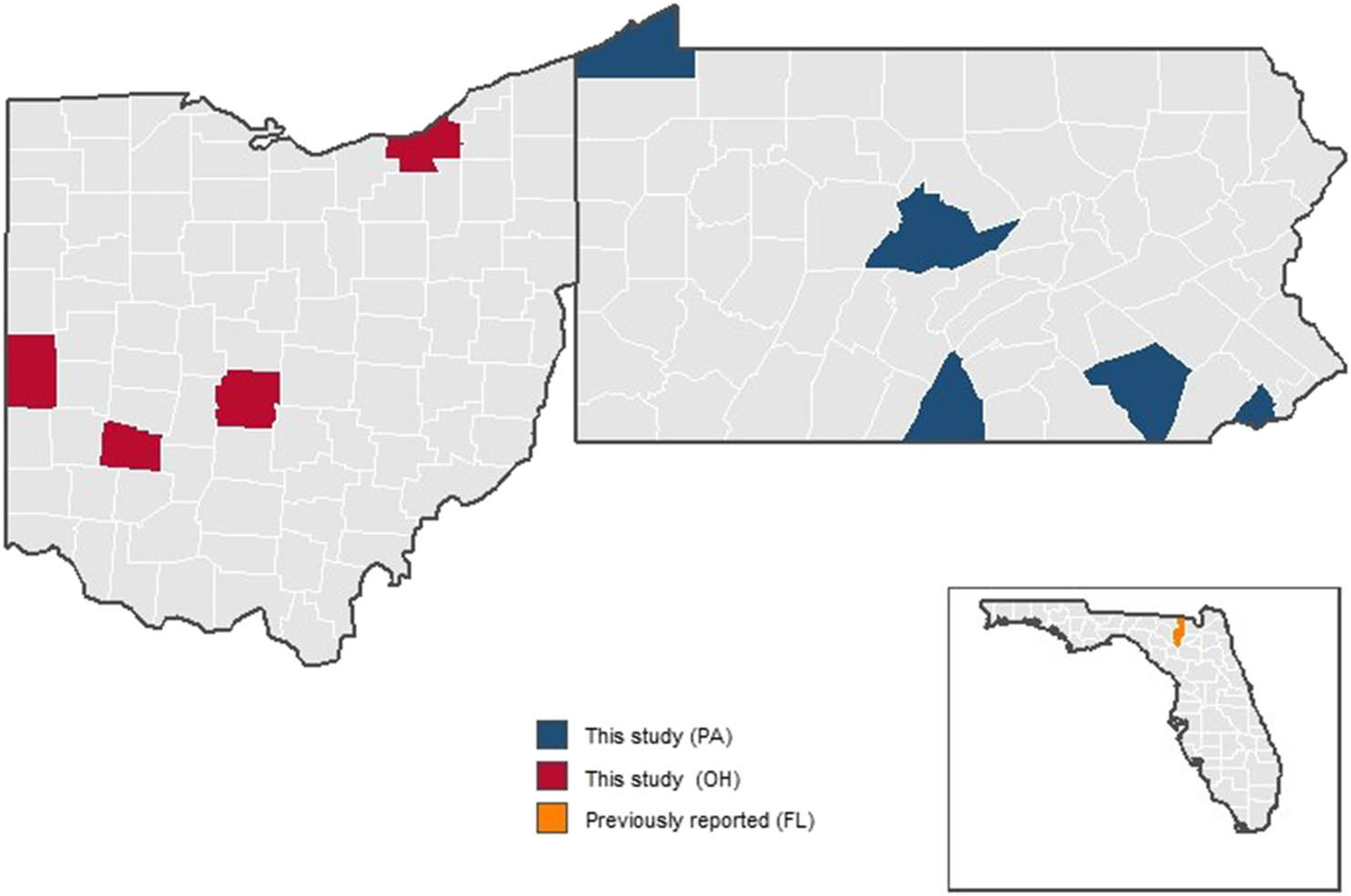
Figure 1
Geographic distribution of Pratylenchus pseudocoffeae in the United States, including new detections in Ohio and Pennsylvania from this study, and a previously reported occurrence in Florida (Inserra et al., 1998).
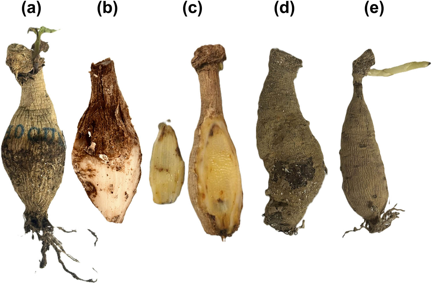
Figure 2
Dahlia tubers submitted to the Pennsylvania State Nematology Laboratory infected with Pratylenchus pseudocoffeae. Panels a and b show the same tuber before and after peeling for nematode extraction; this tuber had a density of 544 P. pseudocoffeae g−1 tuber peel. Panels c–e represent individual infected tubers.
Table 1
Morphometric measurements of Pratylenchus pseudocoffeae recovered from dahlia tubers in Ohio and Pennsylvania, compared with those of type specimens from Japan
| Japan (Topotype) (Mizukubo, 1992) | Ohio, USA | Pennsylvania, USA | ||||
|---|---|---|---|---|---|---|
| Character | (♀) | (♂) | (♀) | (♂) | (♀) | (♂) |
| n | 40 | 11 | 15 | 15 | 10 | 10 |
| L | 554 ± 59.9 | 489 ± 42.7 | 561.1 ± 50.4 (463.3–641.4) | 509.8 ± 23.7 (446.4–552.3) | 555.2 ± 60.0 (500–676) | 472 ± 14.9 (455–492) |
| a | 29.9 ± 2.2 | 30.6 ± 3 | 24.7 ± 2.0 (22.0–29.7) | 28.1 ± 2.9 (21.6–32.6) | 26.8 ± 4.3 (20.0–34.4) | 27.7 ± 3.1 (22.7–31.0) |
| b | 6.3 ± 0.7 | 6.1 ± 0.7 | 4.9 ± 0.6 (4.2–6.3) | 4.7 ± 0.3 (4.4–5.5) | 4.5 ± 0.4 (3.7–5.2) | 4.7 ± 0.3 (4.2–5.13) |
| b′ | 3.1 ± 0.4 | 3.3 ± 0.3 | _ | _ | _ | _ |
| c | 19.4 ± 1.4 | 20.3 ± 1.6 | 21.0 ± 2.2 (17.9–24.8) | 20.6 ± 1.4 (18.4–23.2) | 19.7 ± 2.1 (16.7–24.1) | 20.7 ± 2.4 (18.5–24.6) |
| c′ | 2.3 ± 0.2 | 2.4 ± 0.3 | 1.8 ± 0.2 (1.6–2.1) | 1.9 ± 1.1 (1.6–2.3) | 1.8 ± 0.4 (1.3–2.2) | 2.2 ± 0.6 (1.1–3.1) |
| V (%) | 80.4 ± 0.9 | _ | 80.7 ± 1.5 (79.0–84.0) | _ | 81.2 ± 1.5 (79.5–83.4) | _ |
| Stylet length | 16.4 ± 0.5 | 14.9 ± 0.5 | 14.6 ± 0.6 (13.8–15.9) | 13.6 ± 0.5 (12.3–14.3) | 16.3 ± 0.6 (15.5–17.5) | 15.0 ± 0 15.0–15.0) |
| m (%) | 50.3 ± 1.6 | 50.7 ± 1.9 | 46.3 ± 1.8 (44.1–51.1) | 46.9 ± 0.16 (43.3–50.5) | _ | _ |
| DGO | 1.8 ± 0.39 | 1.8 ± 0.4 | 2.4 ± 0.2 (2.1–2.8) | 2.2 ± 0.2 (1.9–2.9) | _ | _ |
| Knob width | 3.7 ± 0.25 | 3.0 ± 0.2 | 3.5 ± 0.3 (2.8–3.8) | 2.9 ± 0.06 (2.6–3.2) | _ | _ |
| Excretory pore | 88 ± 5.4 | 83 ± 5.7 | 81.1 ± 10 (62.1–98.9) | 82.5 ± 4.8 (75.9–92.1) | 100.1 ± 5.7 (90.5–111.3) | 95.2 ± 11.8 (83.0–119.1) |
| Pharynx | 88 ± 9.1 | 81 ± 8.2 | _ | _ | 83.6 ± 5.1 (77.4–91.1) | 83.8 ± 11.9 (75.4–110.1) |
| Vulva-anus | 80 ± 11.3 | _ | 80.8 ± 11.6(62.9–99.9) | _ | 83.2 ± 6.4 (65.7–102.4) | _ |
| Tail length | 29 ± 3.4 | 24 ± 2.4 | 26.7 ± 2.0 (23.9–29.9) | 23.8 ± 1.1 (22.9–27.7) | 28.5 ± 3.7 (19.0–26.0) | 22.9 ± 2.2 (20.0–25.0) |
| PUS | 28 ± 5.0 | _ | 27.6 ± 3.8 (20.3–34.6) | _ | 27.7 ± 4.4 (22.0–36.0) | _ |
| Tail annuli | 20 ± 1.8 | _ | _ | _ | 22.1 ± 2.5 (19.0–26.0) | _ |
| Spicules | _ | 16.9 ± 1.3 | _ | 17.1 ± 1.1 (15.6–19.4) | _ | 16.6 ± 1.2 (15.0–18.0) |
| Gubernaculum | _ | 4.0 ± 0.4 | _ | 5.4 ± 0.3 (5.1–5.9) | _ | 4.8 ± 0.4 (4.0–5.0) |
| Spicules/stylet ratio | _ | 1.14 ± 0.06 | _ | 1.3 ± 0.08 (1.1–1.4) | _ | 1.1 ± 0.07 (1.0–1.2) |
All measurements are in µm (except ratios) and are presented as mean value ± standard deviation followed by range (min.–max.). Ranges for the Japanese populations were not provided in the original description by Mizukubo (1992).
Abbreviations: n = number of measured specimens; L = overall body length; a = body length/greatest body width; b = body length/pharynx length; c = body length/tail length; c′ = tail length/body width at anus or cloaca; V%: distance of the vulva from the anterior end × 100/total body length; DGO: distance of the dorsal pharyngeal gland orifice from stylet knob base; PUS: post-uterine sac length.
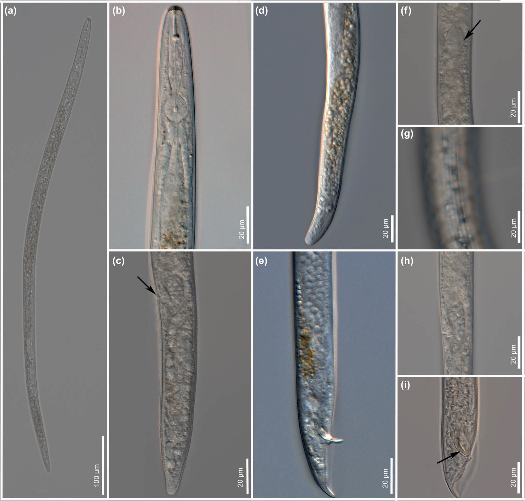
Figure 3
Light micrographs of Pratylenchus pseudocoffeae collected from infected dahlia tubers from Franklin County, Pennsylvania. (a) Female, entire body; (b) female anterior region; (c) female posterior region (arrow indicated vulva position); (d) female posterior end; (e) male posterior end; (f) spermatheca (arrowed); (g) lateral field showing four incisures; (h) vulva region; (i) male reproductive structures (spicules and gubernaculum).
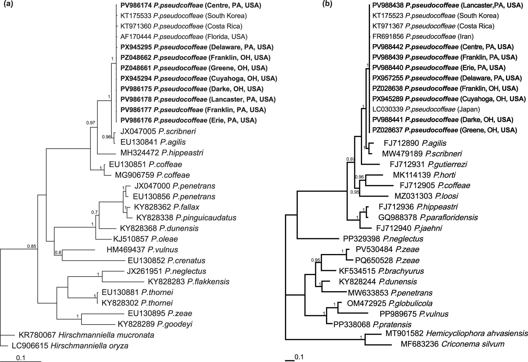
Figure 4
Phylogeny of Pratylenchus pseudocoffeae isolated from dahlia tubers in Ohio and Pennsylvania inferred from the D2D3 region of the 28S (a) and ITS (b) regions of the rDNA. Bayesian analyses employed the GTR + G model. Branch support values above 0.5 are shown as PP next to the respective nodes. Sequences obtained in this study are shown in bold. Outgroup taxa were Hirschmanniella mucronate and H. oryzae for 28S tree; and Hemicycliophora ahvasiensis and Criconema silvum for ITS tree.
Table 2
Summary of root weight, shoot weight, plant height, and nematode population density across treatment levels
| Treatment | n | Mean root weight (g) ± SD | Mean shoot weight (g) | Mean height (cm) | Mean nematode count ± SD |
|---|---|---|---|---|---|
| Control | 4 | 12.96 ± 4.07 a | 9.25 ± 1.23 a | 33.42 ± 2.54 a | 0.0 ± 0.0 a |
| Low | 4 | 3.27 ± 1.76 b | 8.06 ± 3.93 a | 30.41 ± 2.40 ab | 8,204 ± 2019.5 b |
| Medium | 4 | 4.94 ± 3.91 b | 7.40 ± 2.31 a | 27.77 ± 2.11 b | 6,886 ± 3554.6 b |
| High | 4 | 4.40 ± 1.21 b | 6.08 ± 1.04 a | 27.66 ± 1.20 b | 6,708 ± 496.5 b |
Different letters within a column indicate significant differences among treatments according to Tukey’s HD test (α = 0.05).
Abbreviations: n = number of samples; SD = standard deviation.
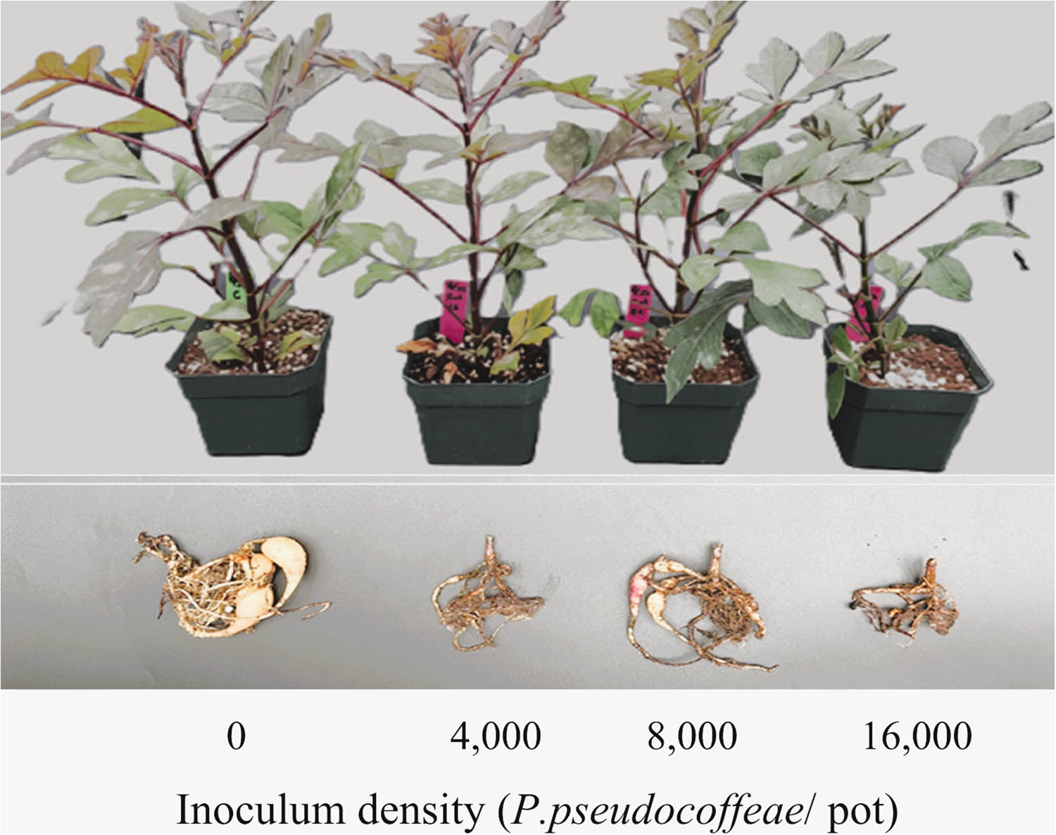
Figure 5
Dahlia plant height at 8 weeks post-inoculation across increasing inoculum densities (0–28 Pratylenchus pseudocoffeae cm−3 soil). Control plants did not receive nematode inoculum. Bottom row shows roots corresponding to each treatment.
Table 3
Dunnett-adjusted reductions and percent reductions in root weight, shoot weight, and plant height for inoculated treatments relative to uninoculated control (n = 4)
| Trait | Contrast | Reduction | Reduction (%) | Lower CL | Upper CL | SE | df | t ratio | P value |
|---|---|---|---|---|---|---|---|---|---|
| Root weight | Low | 9.69 g | 74.8 | 4.01 | 15.38 | 2.13 | 13 | −4.56 | 0.001 |
| Root weight | Medium | 8.02 g | 61.9 | 2.33 | 13.70 | 2.13 | 13 | −3.77 | 0.006 |
| Root weight | High | 8.56 g | 66.1 | 2.33 | 14.79 | 2.33 | 13 | −3.68 | 0.007 |
| Shoot weight | Low | 1.19 g | 12.9 | 2.88 | 5.25 | 1.52 | 13 | −0.78 | 0.757 |
| Shoot weight | Medium | 1.85 g | 20.0 | 2.22 | 5.91 | 1.52 | 13 | −1.22 | 0.500 |
| Shoot weight | High | 3.17 g | 34.2 | 1.28 | 7.62 | 1.66 | 13 | −1.90 | 0.191 |
| Plant height | Low | 3.01 cm | 9.0 | 0.87 | 6.89 | 1.45 | 13 | −2.08 | 0.144 |
| Plant height | Medium | 5.65 cm | 16.9 | 1.77 | 9.53 | 1.45 | 13 | −3.89 | 0.005 |
| Plant height | High | 5.76 cm | 17.2 | 1.51 | 10.01 | 1.59 | 13 | −3.62 | 0.008 |
Statistically significant reductions are indicated in boldface P values.
Abbreviations: df = degree of freedom; CL = Confidence Interval; n = number of samples.