Semantic-Aware Trajectory Planning for UAV in Dynamic Environments

A higher level of autonomy in unmanned aerial vehicles (UAVs) expands their potential for deployment across various real-world applications. This autonomy relies heavily on simultaneous localization and mapping (SLAM) and the capability to generate safe and precise trajectories toward a target.

VI-SLAM systems are widely used in UAVs due to their high accuracy, real-time performance, and autonomy, especially in GPS-denied environments such as indoor spaces or obstructed areas [1–5]. Additionally, for quadrotors with limited payload capacity and battery life, cameras serve as ideal onboard sensors for navigation. However, a key drawback of VI-SLAM is its rapid decline in accuracy when encountering texture-less regions. A common approach to improving accuracy involves keeping specific features or landmarks within the field of view (FOV) [6–8].

Nowadays, the advancements in artificial intelligence (AI), particularly deep learning applied to semantic segmentation [9] and object detection [10], have achieved high accuracy and performance. These techniques enable to label the regions with different characteristics semantically. Semantic information is often incorporated as a term or constraint in optimization frameworks to help avoid textureless or problematic regions, such as lakes and oceans, which can cause significant drift or failures in pose estimation [11,12]. Additionally, it helps prioritize high-textured regions, thereby improving the quality of pose estimation [13–19]. Moreover, semantics have also been employed in the multi-robot planning problem [20].

Ensuring safe arrival at the destination also requires effective obstacle avoidance. However, many existing studies assume the environment is static during collision checking. This limits their deployment in real-world scenarios. Because the real world is exactly the cluttered and dynamic environment.

Common collision-checking methods involve decomposing free space into convex regions such as sequences of axis-aligned cubes [21], convex regions from seeding [22, 23], or creating safe flight corridors (SFC) by inflating pre-existing trajectories (often the global trajectory) [24–28]. Collision-checking can be performed using either discretizing the trajectory into points or outer polyhedral representations. While discretized points are computationally intensive and do not guarantee collision-free paths between sampled points, increasing the number of samples to improve accuracy further adds to the computational burden [29–32].

To reduce the burden of computation, outer representation techniques enclose the trajectory within a polyhedron. If this polyhedron remains inside the free space, the entire trajectory is considered collision-free. For example, in polynomial trajectory optimization [33, 34], it is verified whether the outer polyhedral representation of each trajectory segment is contained within the free space.

A common approach to obtaining this polyhedral representation is by using the convex hull of the control points from the Bernstein or B-Spline basis [35–37]. However, in cluttered and dynamic environments, the free space is significantly reduced. A more compact outer representation improves the likelihood of successful trajectory generation while reducing computational time.

Getting the idea from the prior publications [38–40], this work uses the MINVO basis [41] instead of the Bernstein or B-Spline basis. Depending on the polynomial degree n, MINVO [41] can yield a significantly smaller volume.

Decomposition is especially challenging in cluttered and dynamic environments. In dense environments, it is difficult to construct a tight representation of free space. In dynamic settings, an additional dimension of time makes the decomposition much more complicated, and sometimes it is infeasible. To eliminate the need for decomposition, this work imposes a constraint that verifies the existence of a separating plane between the UAV’s trajectory and obstacle trajectories. This plane constraint is incorporated into the optimization process [38, 40].

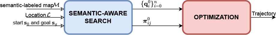
This study presents a novel workflow that guides UAVs to prioritize high-texture areas while avoiding texture-less and hazardous regions in dynamic environments. The proposed approach consists of two main stages: (i) Semantic-Aware Trajectory Initialization, called semantic-aware A* search, prioritizes safe and high-texture areas while avoiding textureless and hazardous regions. The output of this step serves as the initial guess for the second stage. (ii) Dynamic-Aware Optimization accounts for environmental dynamics by combining: (a) Eliminating free space decomposition and replacing it with a separating plane constraint. (b) Utilizing the MINVO basis. At the same time, the trajectory is also energy-optimal and satisfies dynamic constraints.

The UAV is modeled by the geometric shape and state at t. Its shape is a set of vertices in 3D space 𝓥^U = [V₀, V₁,…] ⊂ ℝ³. And the state vector sT(t)=[ xT,x˙T,x¨T ]=[ xT,vT,aT ]{{\bf{s}}^T}(t) = \left[ {{{\bf{x}}^T},{{{\bf{\dot x}}}^T},{{{\bf{\ddot x}}}^T}} \right] = \left[ {{{\bf{x}}^T},{{\bf{v}}^T},{{\bf{a}}^T}} \right], where x, v and a are the position, velocity and acceleration, respectively.

The environment in which the UAV operates is a cluttered and dynamic environment. It is modeled by a metric-semantic map ℳ. It consists of unknown regions ℳ_unknown and known regions ℳ_known. These known regions contain static obstacles 𝒪_static, dynamic obstacles 𝒪_dyn and the regions which semantically-labelled as texture-high ℳ_att or hazardous/texture-less ℳ_rep. So ℳ = ℳ_unknown ∪ 𝒪_dyn ∪ 𝒪_static ∪ ℳ_att ∪ ℳ_rep.

At this time, the problem is how to generate a feasible trajectory that guides the UAV from the initial state s₀ to the goal state s_g safely and accurately within the environment ℳ, while ensuring the minimization of control energy by leveraging the semantic information available in that semantic map.

To solve this problem, several key subproblems need to be addressed as follows:

• -

  subproblem 1: Defining the trajectory.

• -

  subproblem 2: HOW TO check collision in cluttered and dynamic environment even during trajectory generation. Details are presented in section 3 below.

• -

  subproblem 3: HOW TO leverage semantic information to improve the process of trajectory generation for a certain purpose, more detailed in section 4.

• -

  subproblem 4: Formulating and solving the programming optimization. It is described in more detail in section 5.

We use the method of polynomial trajectory planning [28, 33] with clamped uniform B-Splines. So, the UAV’s trajectory x(t):=[x(t),y(t),z(t)]T=∑k=0nBk,p(t)qk{\bf{x}}(t): = {[{\rm{x}}(t),{\rm{y}}(t),{\rm{z}}(t)]^T} = \sum\nolimits_{k = 0}^n {{B_{k,p}}} (t){{\bf{q}}_k} is defined by n + 1 control points {q₀,…, q_n} and m + 1 knots {t₀, t₁, …, t_m}. Its each segment is a p-degree B-spline function and indexed by j (j ∈ J, J is the total number of intervals) starting from 0 (As described in Fig. 2, j = 0, …, m − 2p − 1). In total, it has m − 2p − 1 intervals. It is clamped to ensure that it passes through s₀ (the first p + 1 knots are identical) and s_g (the last p + 1 knots are identical). The knots between the first p + 1 and the last p + 1 knots are called internal knots. The uniform means that the internal knots are equally spaced.

Figure 1.

Workflow of semantic-aware trajectory planning including two consecutive steps. They are semantic-aware search and optimization, described in section 4 and 5, respectively

Figure 2.

The problem of UAV trajectory planning in a cluttered and dynamic environment. The trajectory is generated portion by portion to ensure real-time performance and feasibility

In this paper, we use the cubic splines (i.e., p = 3). This balances the dynamic feasibility of a UAV and computational efficiency [40]. So, the input control u(t) is jerk j(t) and itis constant at the same interval j(j) = const.

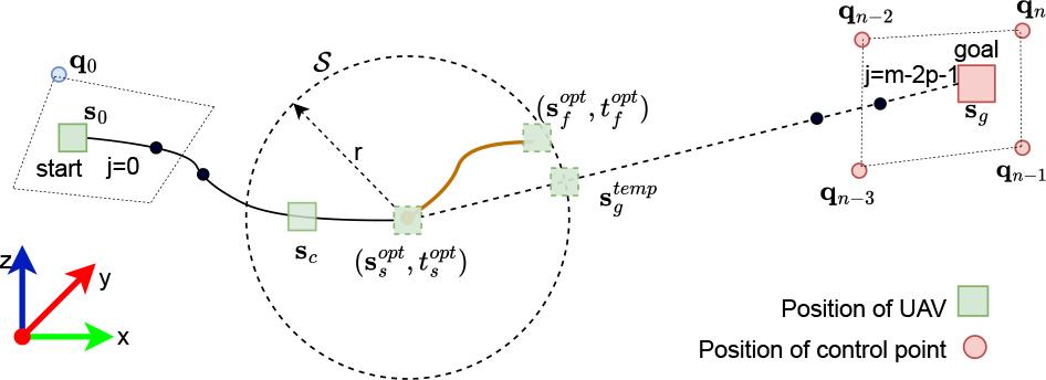
To ensure the real-time performance and feasibility, the consuming time of trajectory generation needs to be limited within a time interval of δ(t). This is achieved by generating only the portion of the trajectory (illustrated by Fig. 2, it is the golden-brown segment) that lies within a sphere 𝒮 with the radius r. During re-planning, r remains fixed. The trajectory generation starts at a time when UAV is staying at s_c and at the moment before the time of completing the execution of the previous portion of the trajectory by δ(t) (illustrated in Fig. 2).

Thus, at this point, the starting point is the moment when the execution of the previous portion of the trajectory is completed tsoptt_s^{opt}, corresponding to state ssopts_s^{opt}. The goal of the trajectory is no longer s_g but instead a temporary target sstemps_s^{temp}. This temporary target is obtained by the intersection between sphere 𝒮 and a piece-wise linear path that goes from (ssopt,tsopt)\left( {s_s^{opt},t_s^{opt}} \right) that avoids the static obstacles. The final target of the resulting portion is sfopts_f^{opt} at time tfoptt_f^{opt}, which does not necessarily coincide with sgtemps_g^{temp}. Next, we delve into the details of solving the remaining subproblems.

As described in section 1, to alleviate the burden of computing, All of the trajectories are represented by outer polyhedrals. And then checking whether or not the intersection of them for collision.

3.3.

Collision Checking

In subsection 3.2, the convex hull of the obstacles has already accounted for the UAV’s size, so the UAV is now treated as a point of mass. This means that the UAV and the obstacle do not collide if the MINVO convex hull QjMVQ_j^{MV} (computed in subsection 3.1) of the UAV’s trajectory does not intersect with the convex hull of the obstacle 𝓒_ij (computed in subsection 3.2).1{ nijTc+dij>0,∀c∈Cij,∀i∈I,j∈JnijTq+dij<0,∀q∈QjMV,∀j∈J\left\{ {\matrix{ {{\bf{n}}_{ij}^T{\bf{c}} + {d_{ij}} > 0,} \hfill & {\forall {\bf{c}} \in {{\cal C}_{ij}},\forall i \in I,j \in J} \hfill \cr {{\bf{n}}_{ij}^T{\bf{q}} + {d_{ij}} < 0,} \hfill & {\forall {\bf{q}} \in {\cal Q}_j^{{\rm{MV}}},\forall j \in J} \hfill \cr } } \right. where:

• –

  n_ij is the normal vector defining the separating hyperplane.

• –

  d_ij is a bias term shifting the hyperplane.

• –

  𝓒_ij is the convex region representing the obstacle.

• –

  QjMV{\cal Q}_j^{MV} is the convex region representing the UAV trajectory (using the MINVO basis).

• –

  I is the total number of obstacles.

• –

  J is the set of UAV trajectory intervals.

In other words, they do not collide if there exists a separating hyperplane π_ij (characterized by the normal vector n_ij and bias d_ij) between their convex hulls, described by Eq.1. The first inequality of Eq.1 ensures that all points c in the obstacle set 𝓒_ij lie on one side of the plane. The second one ensures that all points q in the UAV’s trajectory set QjMV{\cal Q}_j^{MV} lie on the other side.

An illustration of an outer polyhedral representation and collision-checking that includes static and dynamic obstacles, as well as UAV is shown in Fig. 3. Fig. 3a illustrates all of the convex hulls and collision checking at the first and second intervals. Fig. 3b and 3c illustrate the convex hull and collision checking at the third and fourth intervals, respectively. This problem is solved using GLPK [43] or Gurobi [44].

Figure 3.

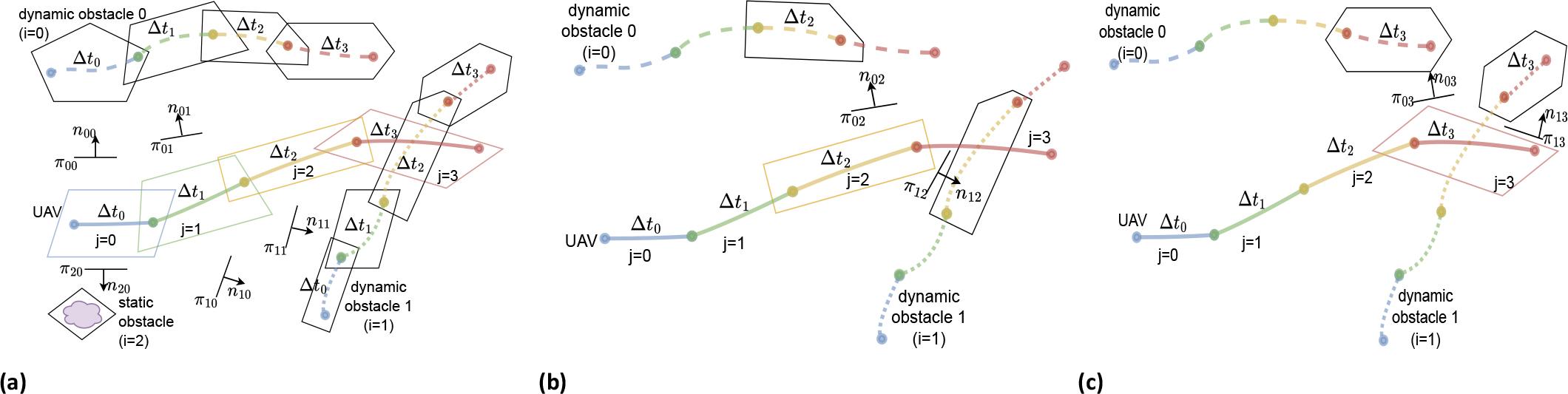
Outer representation of trajectories of UAV, dynamic obstacles (for instance, obstacle 0 and 1), static obstacle (for example, obstacle i = 2) and Collision-checking by separating planes π_ij: (a) Collision-checking at the 1^st and 2^nd interval of UAV trajectory. (b) Collision-checking at the 3^rd interval of UAV trajectory.(c) Collision-checking at the 4^th interval of UAV trajectory

This algorithm is inspired by the original A* [45] for path-finding based on not only traditional costs but also the semantic information about the environment. In particular, its resulting path is to prioritize the rich-informative regions while avoiding hazardous or low-informative areas. So itis called as semantic-aware A*. This is achieved by introducing additional cost values into the total cost function f. Each MINVO control point serves as a node in the search. All open nodes are maintained in a priority queue openSet, where elements are ordered in ascending order off.

With semantic-labeled map ℳ, the regions with high information tend to attract the UAV, modeled by C_att. Whereas the hazardous or low-informative regions tend to repel the UAV, modeled by C_rep (described in Fig. 5).2f(.)=λgg(.)+λhh(.)+λattCatt(.)−λrep Crep (.)f(.) = {\lambda _{\rm{g}}}g(.) + {\lambda _{\rm{h}}}h(.) + {\lambda _{{\rm{att}}}}{C_{{\rm{att}}}}(.) - {\lambda _{{\rm{rep }}}}{C_{{\rm{rep }}}}(.)

Figure 4.

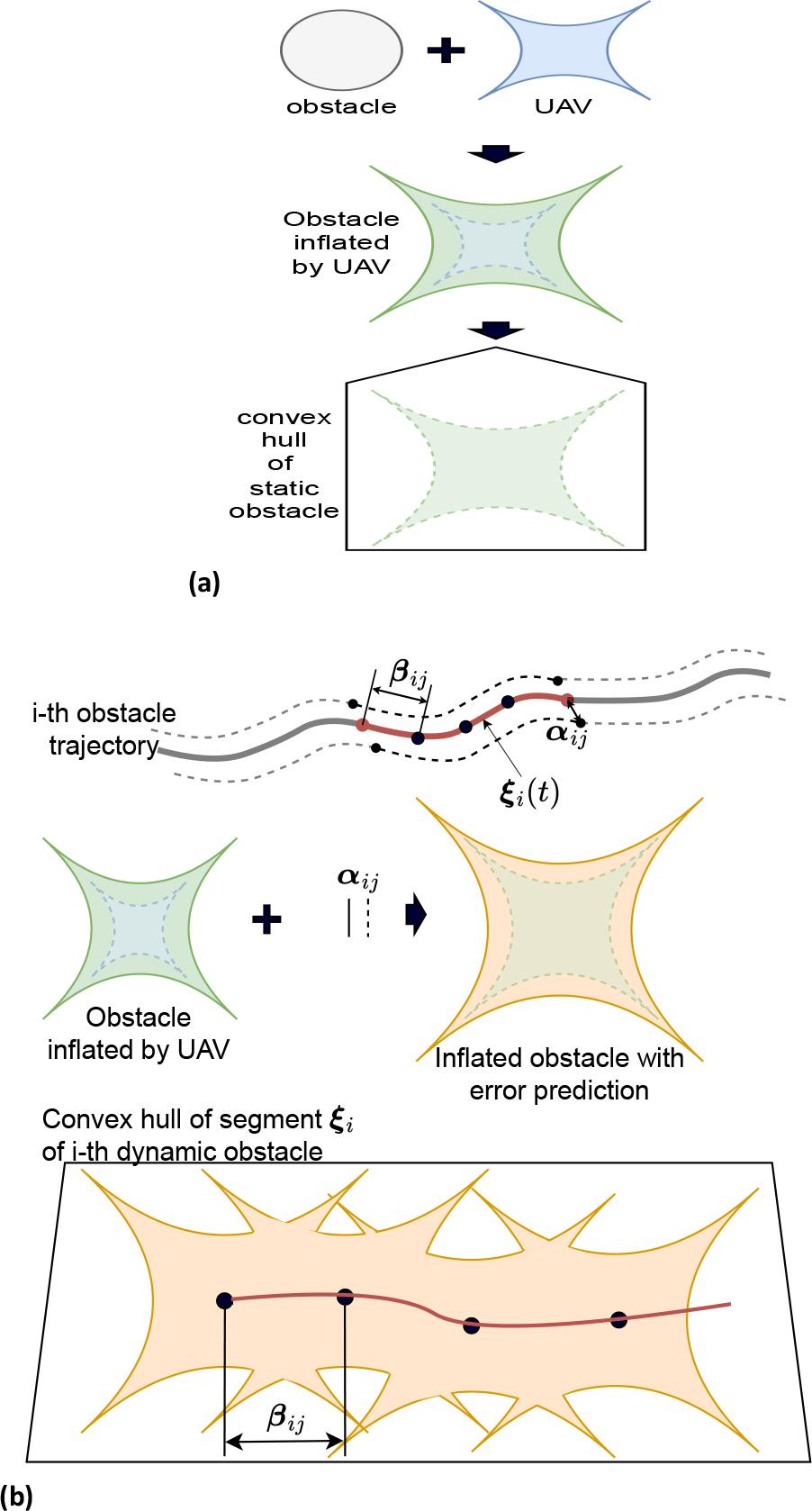
Outer representation of the obstacles: (a) For static obstacle. (b) For dynamic obstacle

Figure 5.

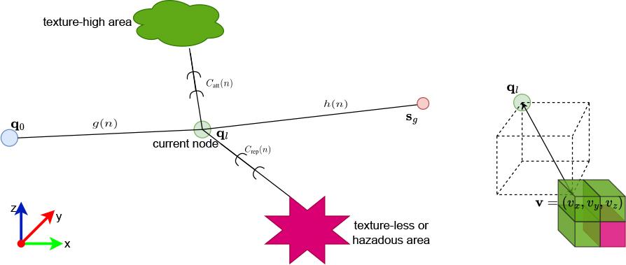
The total cost of semantic-aware A* includes traditional costs, along with repulsive and attractive costs arising from texture-less/hazardous regions (vivid pinkish-magenta color) and high-texture areas (fresh green color), respectively. Along with HOW TO calculate the Euclidean distance in 3D space used as primitive for calculating the costs

So, at this time, the total cost function f(.) includes four terms, where g(.) is the sum of the distances (between successive control points) from q₀ to the current node q_l (cost-to-come), h(.) is the distance from the current node q_l to the goal s_g (heuristics of the cost-to-go), C_rep(.) is for repelling UAV away from the low-texture regions, while conversely, C_att(.) is for attracting towards informative areas, as modeled in Eq. 2.

The position of each voxel in the map ℳ is vvx=(vxvx,vyvx,vzvx){{\bf{v}}^{vx}} = (v_x^{vx},v_y^{vx},v_z^{vx}), so v^vx ∈ ℳ. Let ℳ_att, ℳ_rep ⊆ ℳ be the set of all voxels in the attractive and repulsive regions, respectively. The cost value of these two regions (ℳ_att and ℳ_rep) is calculated as the sum of the distances from the current control point q_l to all the voxels in that region.

However, their influence on the total cost (according to Eq. 2) is opposite. By increasing the total cost, C_att prioritizes regions with smaller distances. In contrast, C_rep decreases the total cost, thereby prioritizing regions with larger distances, meaning it tends to push the trajectory away from those regions. They are calculated by Eq. 3, where the sign “_” indicates att or rep.3C−(.)≔1| ℳ− |∑vvx∈ℳ−d(ql,vvx){C_ - }(.): = {1 \over {\left| {{{\cal M}_ - }} \right|}}\sum\limits_{{{\bf{v}}^{vx}} \in {{\cal M}_ - }} d \left( {{{\bf{q}}_l},{{\bf{v}}^{vx}}} \right)

The weights λ_g, λ_h, λ_att λ_rep ∈ ℝ⁺ in Eq. 2 determine the influence of each component on the total cost f(·) If a weight is greater than 1, the corresponding component has a stronger influence (for example, if λ_att > 1, the trajectory is more strongly guided toward the attractive region). On the other hand, when the weight is less than 1 (0 < λ < 1), the corresponding component has a weaker influence compared to the others. If the weight equals 1, it has a balanced influence according to its original value.

The algorithm is represented as a pseudo-code in Alg. 1. Firstly, control points q₀, q₁, q₂ is determined from the initial state ssopts_s^{opt} at the moment tsoptt_s^{opt} (line 1). At the starting moment t₀, we have tsopt=t0t_s^{opt} = {t_0} and ssopt=s0s_s^{opt} = {s_0}. And then it initializes the openSet queue, gCost and fCost (line 2 to 5).

The loop of semantic-aware A* search is run until openSet queue is empty or out of time: The first item, which is with f value is lowest, is popped (line 7) and remove it (line 14) if it simultaneously does not touch the target (line 8) and satisfies some conditions (line 16). The search process is considered complete if q_l is within a predefined distance ϵ from the intermediate goal sgtemps_g^{temp} and it’s index l = n − 2 (line 8). Since the velocity v and acceleration a of the UAV are zero when it reaches the final target s_g, it follows that q_n-2 = q_n-1 = q_n. The result will be a sequence of control points { qi }i=0n\{ {{\bf{q}}_i}\} _{i = 0}^n, which come from inferring the sequence from q₀ to q_n-2 (line 9) backward and appending two ending points (line 10 and 11), and hyperplanes π_ij that separate them from obstacles.

For q_l node to be accepted, it must satisfy several conditions (line 16): it must be inside the sphere S(‖ ql−ssopt ‖2≤r){\cal S}({{\bf{q}}_l} - {\bf{s}}_s^{opt}{_2} \le r) as stated in section 2, not be too close to another q_k already in the openSet (||q_l − q_k||_∞ > δ) to alleviate the burden of computing, and obviously not collide (isCols is false). The collision is checked by determining which QjMV{\cal Q}_j^{MV} contains q_l, then solving Eq. 1 (details in subsection 3.3).

The result is a hyperplane added to π_ij and a binary variable isCols indicating whether or not a collision occurs (line 15).

Next, the best neighbor of q_l is expanded and added to openSet queue: For each value of Δv, which is uniform-sampled ensuring the limits v_max and a_max. The neighbor is computed (line 20) using a time step of Δt/p where Δt=‖ ssopt −sgtemp ‖2vmax\Delta t = {{{\bf{s}}_s^{opt{\rm{ }}} - {\bf{s}}_g^{temp{\rm{ }}}{_2}} \over {{{\bf{v}}_{\max }}}}. The best neighbor is selected, and if it is not already in the openSet, it is added (lines 22 to 27), while its fCost value is evaluated (line 25). Moreover, if the search time exceeds the predefined limit (that is timeout), it will return the sequence of control points, which is with the last point being the closest to the intermediate goal sgtemps_g^{temp}, and it’s corresponding hyperplanes π_ij (line 32). This algorithm is tested in subsection 6.1 below.

Based on the initial trajectory (converted from [ { qi0 }i=0n,πij0 ][\{ {\bf{q}}_i^0\} _{i = 0}^n,{\bf{\pi }}_{ij}^0]) getting from semantic-aware A*. We need to smooth and make it feasible by programming optimization with the goal of minimizing energy consumption and reaching the target as closely as possible. This problem is parameterized by control points QjBSQ_j^{BS} and planes variables π_ij(n_ij, d_ij). It minimizes the energy consumption through control input ∫tsopttfopt‖u(t)‖2dt=∫tsopttfopt‖j(t)‖2dt=∑j∈J‖j(j)‖2\mathop \smallint \limits_{t_s^{opt}}^{t_f^{opt}} {\bf{u}}(t){^2}dt = \mathop \smallint \limits_{t_s^{opt}}^{t_f^{opt}} {\bf{j}}(t){^2}dt = \mathop \sum \limits_{j \in J} {\bf{j}}(j){^2} And the target is reached as closely as possible in terms of distance ‖ qn−sgtemp ‖2{{\bf{q}}_n} - {\bf{s}}_g^{temp}{_2}. Because of q_n–2 = q_n–1 = q_n, it should be ‖ qn−2−sgtemp ‖2{{\bf{q}}_{n - 2}} - {\bf{s}}_g^{temp}{_2}. This is modelled by Eq. 4.minQjBS,nij,dijωu∑j∈J‖j(j)‖2+ωg‖ qn−2−sgtemp ‖22\mathop {\min }\limits_{{\bf{Q}}_j^{{\rm{BS}}},{{\bf{n}}_{ij}},{d_{ij}}} {\omega _u}\sum\limits_{j \in J} {{\bf{j}}(} j){^2} + {\omega _g}\left\| {{{\bf{q}}_{n - 2}} - {\bf{s}}_g^{{\rm{temp }}}} \right\|_2^2 subjects to: 4(i)ss(tsopt)=ssopt,(ii)v(tgopt)=0,a(tgopt)=0,(iii){ nijTc+dij>0,∀c∈𝓒ij,∀i,j,nijTq+dij<0,∀q∈QjMV,∀i,j, (iv)‖ q−ssopt ‖22≤r2,∀q∈QjMV,∀j,(v){ |v|≤vmax,∀v∈VjMV,∀j,| al |≤amax,∀l∈L\{n−1,n}\matrix{ {{\rm{(i)}}} \hfill & {{{\bf{s}}_s}\left( {t_s^{opt}} \right) = {\bf{s}}_s^{opt}} \hfill \cr {{\rm{(ii)}}} \hfill & {{\bf{v}}\left( {t_g^{opt}} \right) = {\bf{0}},\quad {\bf{a}}\left( {t_g^{opt}} \right) = {\bf{0}},} \hfill \cr {{\rm{(iii)}}} \hfill & {\left\{ {\matrix{ {{\bf{n}}_{ij}^T{\bf{c}} + {d_{ij}} > 0,} \hfill & {\forall {\bf{c}} \in {{\cal C}_{ij}},\forall i,j,} \hfill \cr {{\bf{n}}_{ij}^T{\bf{q}} + {d_{ij}} < 0,} \hfill & {\forall {\bf{q}} \in {\cal Q}_j^{{\rm{MV}}},\forall i,j,} \hfill \cr } } \right.} \hfill \cr {{\rm{(iv)}}} \hfill & {\left\| {{\bf{q}} - {\bf{s}}_s^{opt}} \right\|_2^2 \le {r^2},\quad \forall {\bf{q}} \in {\bf{Q}}_j^{{\rm{MV}}},\forall j,} \hfill \cr {{\rm{(v)}}} \hfill & {\left\{ {\matrix{ {|{\bf{v}}| \le {{\bf{v}}_{\max }},\quad \forall {\bf{v}} \in {\cal V}_j^{{\rm{MV}}},\forall j,} \hfill \cr {\left| {{{\bf{a}}_l}} \right| \le {{\bf{a}}_{\max }},\quad \forall l \in L\backslash \{ n - 1,n\} } \hfill \cr } } \right.} \hfill \cr }

This problem subjects to some constraints:

• (i)

  The starting point of this inverval is the endpoint of previous one. That is, s(tsopt)=ssopt{\bf{s}}(t_s^{opt}) = {\bf{s}}_s^{opt} as describled in detail in section 2. Obviously s_s(0) = s₀.

• (ii)

  When s_g is inside the sphere 𝒮, it means that the last segment of trajectory is optimized (that is, j = m − 2p − 1 or s(tgopt)=sg{\bf{s}}(t_g^{opt}) = {{\bf{s}}_g}). The UAV’s velocity v(tgopt)=0{\bf{v}}(t_g^{opt}) = {\bf{0}} and acceleration a(tgopt)=0{\bf{a}}(t_g^{opt}) = {\bf{0}}.

• (iii)

  Ensuring the safety (collision-avoiding) in a dynamic environment, detailed in subsection 3.3.

• (iv)

  Guaranteeing that the generated segment of trajectory remains inside sphere 𝒮, detailed in section 2.

• (v)

  The trajectory must comply with kinematic constraints. Specifically, velocity and acceleration must not exceed UAV’s physical limits v_max and a_max, respectively. Because the trajectory is represented by B-Splines, which is a continuous function of time. So directly imposing these constraints (v_max, a_max) at every single point in time along this continuous trajectory would lead to an infinite number of constraints, making the optimization problem computationally intractable.

Moreover, the control points q parameterize the entire trajectory segment. Therefore, by placing constraints on these control points (velocity v and acceleration a), we can indirectly influence and bound the physical velocity and acceleration throughout the interval. The bound of the velocity v_max and acceleration a_max of control points are inferred the physical ones, respectively. This problem (Eq. 4) is solved by Gurobi [44].

In the experiments, we use the configuration of the system as following:

• -

  Hardware: 16 cores Intel Core i7-10875H @ 2.30GHz; GPU Nvidia TU117GLM [Quadro T1000 Mobile]; RAM memory of 32 GB.

• -

  Software: Ubuntu 20.04 LTS; ROS noetic [46] serves as the middleware framework for communication between the planner, simulator, and visualization/logging tools. It provides standardized message passing and modular integration of different software components.

For all planning and collision checking, the UAV is modeled as a sphere of radius r_UAV = 0.1 (m) which upper-bounds the vehicle body and rotor sweep. While rotor disks are omitted in the figures for visual clarity, this inflated model guarantees safe clearance in all experiments. To guarantee real-time performance and feasibility, the planning horizon is limited to a sphere of radius r = 4.0 m, as detailed in Section 2.

Moreover, to focus on the trajectory planning algorithms, it is assumed that the UAV can perfectly track the trajectories generated by the planner.

6.1.

Testing semantic-aware A* solely

This section evaluates the semantic-aware A* algorithm (presented in section 4) in two aspects: the influence of semantic information and the avoidance of dynamic obstacles with the following configuration: λ_g = 1.0, λ_h = 1.0, runtime = 0.1 second, degree of B-spline = 3 (cubic b-spline), number of segments = 6 and one trefoil-knot-based dynamic obstacle.

The trajectory of the dynamic obstacle, ξ(t), is modeled as a trefoil knot [47, 48]. Although the trefoil knot does not reflect realistic obstacle motion, it provides several advantages:

• (i)

  Challenging yet structured – its 3D, non-trivial trajectory is more demanding than linear or circular paths, making it a strong test for collision avoidance.

• (ii)

  Repeatable – its mathematical definition ensures identical, reproducible runs.

• (iii)

  Controlled complexity – the trajectory is well understood, enabling systematic evaluation of algorithm performance.

• (iv)

  Visually distinct – its clear shape facilitates observation and validation in simulations.

The first case considers no influence of semantic information with λ_att = 0, λ_rep = 0. In this case, the search process tends toward the goal while avoiding obstacles (Fig. 6a). In the second case, testing the algorithm in an environment containing a texture-high region (the green area in Fig. 6c and 6d) with λ_att = 2.0, λ_rep = 0. The experimental results in Fig. 6c show that the search process tends to shift toward the texture-high region compared to the first case. The third case examines the algorithm in an environment with a texture-less or unsafe region (the red area in Fig. 6e and 6f) with λ_att = 0,λ_rep = 0.5. The results indicate that the search process tends to avoid this region.

Figure 6.

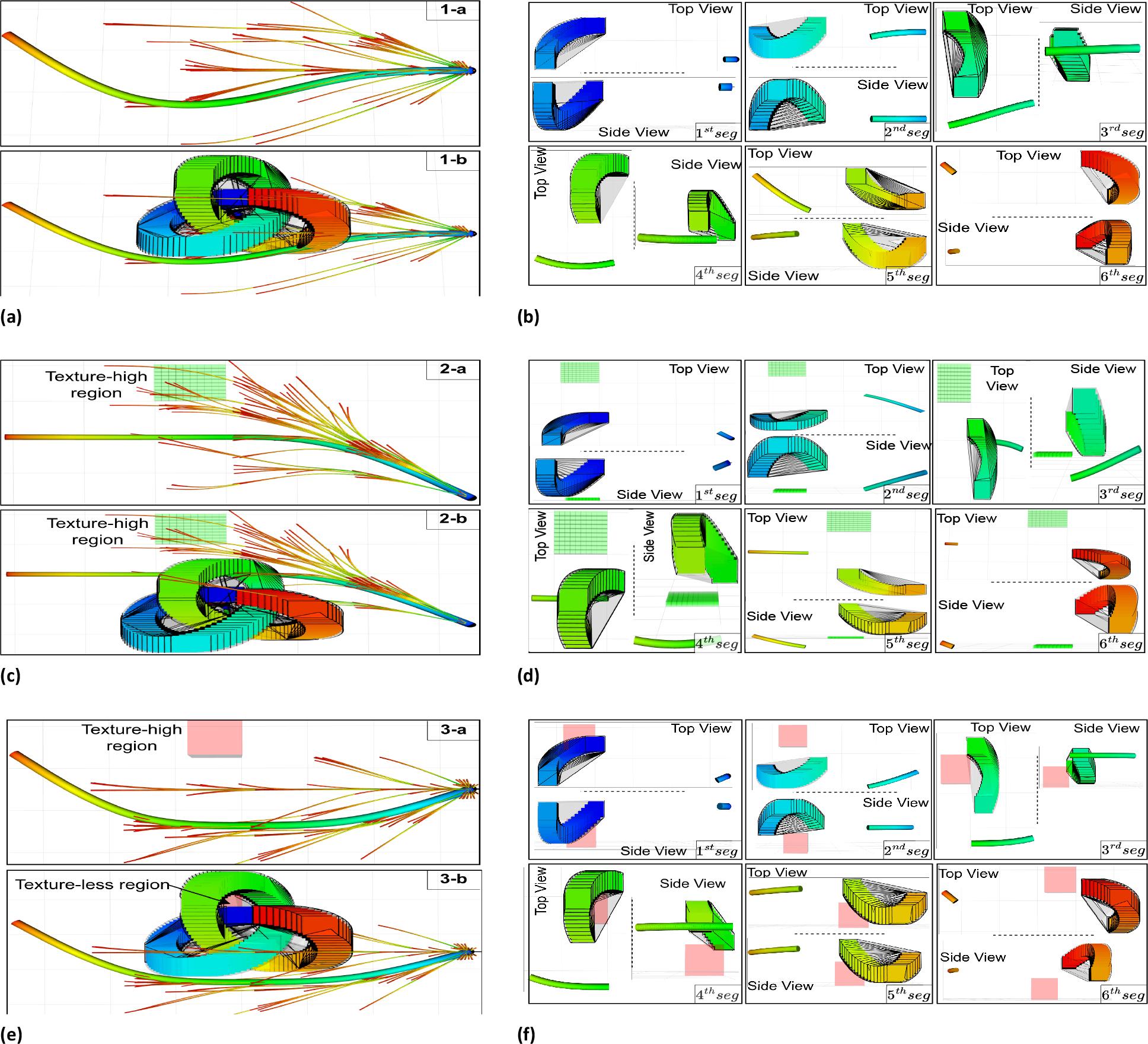
The experimental results of semantic-aware A* with one dynamic obstacle in three cases (Without semantics, Considering the influence of the attractive region and Considering the influence of the repulsive region): (a), (c), and (e) show the complete trajectories, while (b), (d), and (f) display the corresponding individual trajectory segments (1-6) for each case

In all of these cases, the results in (Fig. 6b, 6d and 6f) show that dynamic obstacle avoidance is fully ensured at each segment (from 1^st to 6^th one). Because the obstacles are still considered to be in motion (no temporarily-static) during the collisionchecking process. The experimental results (Figure 6) demonstrate that the proposed semantic-aware A* algorithm behaves as expected, showing a tendency to move toward regions rich in information while avoiding information-poor areas.

6.2.

Experiment with cluttered and dynamic environment

In this section, we evaluate the system’s capability to simultaneously leverage the semantic information – both to avoid and/or to prioritize traversing certain regions – while operating in a dynamic environment, by comparing it with the MADER system [38], which does not utilize semantic information. The evaluation is conducted in a dynamic environment measuring 70 x 4.0 x 4.0 meters (Fig. 7a and 7d), where 65% of the obstacles are dynamic – represented by red cubes, each sized 0.8 x 0.8 x 0.8 (m) – while the remaining 35% are static obstacles, depicted as blue rectangular boxes, each measuring 0.4 x 0.4 x 8.0 (m).

Figure 7.

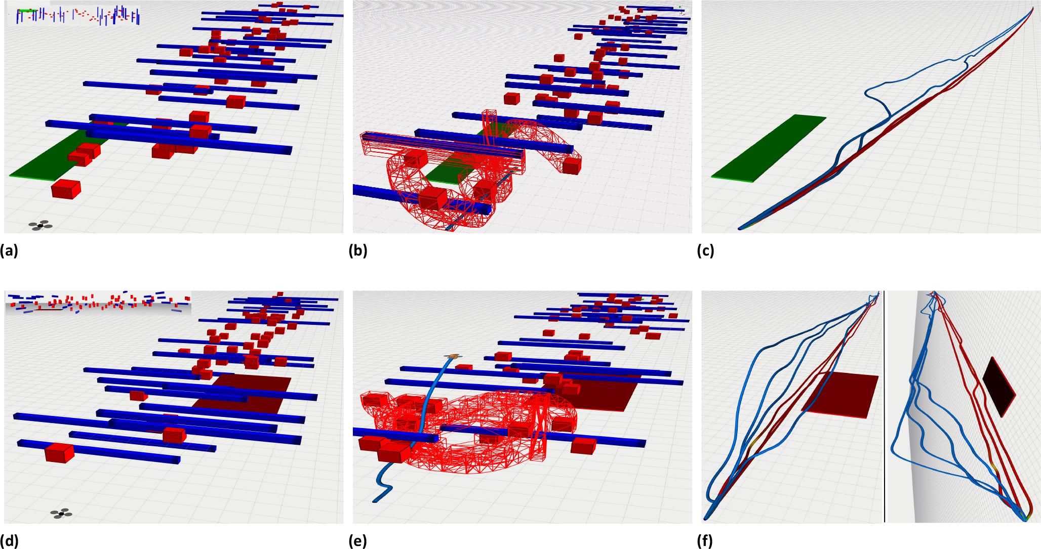
Experiments in dynamic corridor environment: (a) The environment includes dynamic and static obstacles (the red cube and the blue rectangular box, respectively), as well as a rich-information region (the green rectangular box); (b) The quadrotor flies in a dynamic environment, with outer polyhedra (red boxes) surrounding obstacles; (c) The dark blue and dark red trajectories come from our suggestion and MADER [38], respectively; (d-f) The corresponding setup, flight, and trajectory results for a scenario including a low-texture or hazardous region (red rectangular box)

Two simulation scenarios are conducted. The first features a dynamic environment containing a high-texture region, visually indicated by a green rectangle (Fig. 7a, 7b and 7c). The second includes a poortexture or hazardous region, represented by a red rectangle. Both scenarios share the same UAV dynamic constraints, with a maximum velocity of v_max = [6.0 6.0 6.0] m/s and a maximum acceleration of a_max = [20 20 10] m/s², corresponding to the velocity and acceleration limits, respectively. Additionally, in the first scenario, the goal position is set to (75.0, −10.0, 1.0) m, whereas in the second scenario, it is set to (75.0, −1.0, 1.0) m. The runtime of the MILP phase is bounded between 0.05 and 0.35 second.

In the first scenario, simulations are conducted by MADER [38] and our suggession (λ_att = 2.0), followed by a comparison of the resulting trajectories. The simulation results show that the UAV is capable of navigating safely in a dynamic environment (Fig. 7b), while also exhibiting a tendency to pass through the high-texture region (the dark blue trajectory in Fig. 7c).

Similarly, in the second scenario, considering the low-texture or hazardous area corresponds to λ_rep = 2.0. The resulting trajectory shows that the UAV tends to avoid these regions (the dark blue trajectory in Fig. 7f), while still successfully reaching the goal within the dynamic environment (Fig. 7e).

This work introduces a complete workflow for semantic-aware trajectory planning that enables UAVs to navigate autonomously in cluttered, dynamic environments while simultaneously exploiting semantic information to prioritize or avoid specific regions depending on task objectives. Compared to non-semantic planners (such as MADER), which do not leverage semantics, our approach achieves more efficient and context-aware navigation, with trajectories that tend to avoid hazardous zones and approach information-rich regions.

The proposed approach combines a semantic-aware A* initialization, which biases trajectories toward safe and informative regions, with a dynamic-aware optimization that refines the path using separating plane constraints and the MINVO basis while ensuring energy efficiency and dynamic feasibility.

Nevertheless, several limitations remain. The optimization currently considers only the UAV’s position and not its orientation, which may constrain applicability in tasks requiring viewpoint control. Our simulations also do not yet report quantitative state-estimation errors under semantic versus non-semantic settings, and dynamic obstacles are assumed to follow known trajectories rather than stochastic, uncertain motions.

Concrete directions for future work include extending the formulation to explicitly handle UAV orientation and perception-aware objectives, incorporating online estimation of dynamic obstacle motion with uncertainty, and validating the approach in hardware experiments with real UAVs. Another promising direction is to adapt or learn the semantic weights (λ_att, λ_rep) online using reinforcement or imitation learning, thereby tailoring behavior to specific missions while maintaining robustness.

Overall, this work represents a first step toward bridging high-level semantic understanding with low-level dynamic feasibility, paving the way for safer and more intelligent UAV autonomy in complex real-world environments.