

Table 1.
Comparison of AMRs and AGVs
| Feature | AMRs | AGVs |
|---|---|---|
| Navigation Technology | AI-driven sensor-based navigation (LiDAR, cameras, millimeter-wave sensing) [17] | Follow fixed paths using magnetic strips, beacons, or QR codes [18] |
| Path Dependency | No predefined paths; dynamically plans routes in real-time [17] | Fixed paths with minimal deviation from predefined routes [18] |
| Environmental Adaptability | Highly adaptable to unstructured and dynamic environments [17,19] | Limited to structured environments with predefined routes [18] |
| Obstacle Detection | Advanced AI-based obstacle detection with real-time path adjustments [20] | Basic obstacle detection; usually stops when encountering obstacles [18] |
| Operational Flexibility | High flexibility; can navigate new environments without pre-set guides [21] | Low flexibility; requires infrastructure modification for route changes [21] |
| Implementation Cost | Higher initial investment due to advanced sensing and AI [22] | Lower initial investment but higher cost for infrastructure setup [22] |
| Application Suitability | Smart factories, adaptive logistics, and warehouses [17,18] | Manufacturing lines, repetitive logistics, and controlled environments [17] |
| Path-Planning Algorithms | Hybrid A*, RRT, D*, and reinforcement learning-based methods [23] | Mostly rule-based or fixed path-following algorithms [23] |
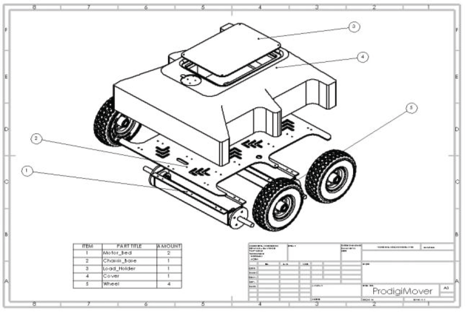
Figure 1.
Exploded 3D model of mobile transportation robot
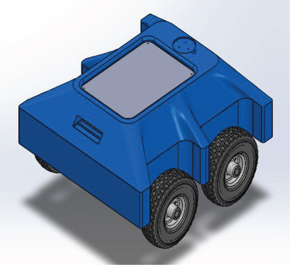
Figure 2.
3D model view of mobile transportation robot
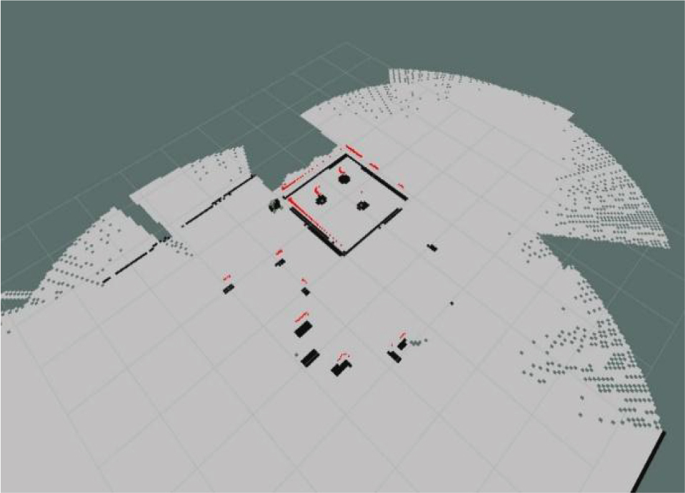
Figure 3.
Creation of map by slam_gmapping node according to real-world environment
Table 2.
DC motor general specifications
| General Specifications | |
|---|---|
| Rated voltage | 12 V |
| Size | 37D × 70L mm |
| Shaft diameter | 6 mm |
| Gear ratio | 70:1 |
| Speed without load | 150 rpm |
| Speed at max. efficiency | 130 |
| Current without load | 0.2 A |
| Current at max. efficiency | 0.68 A |
| Stall torque | 27 kg/cm |
| Torque at max. efficiency | 32 kg/cm |
| Encoder resolution | 64 CPR |
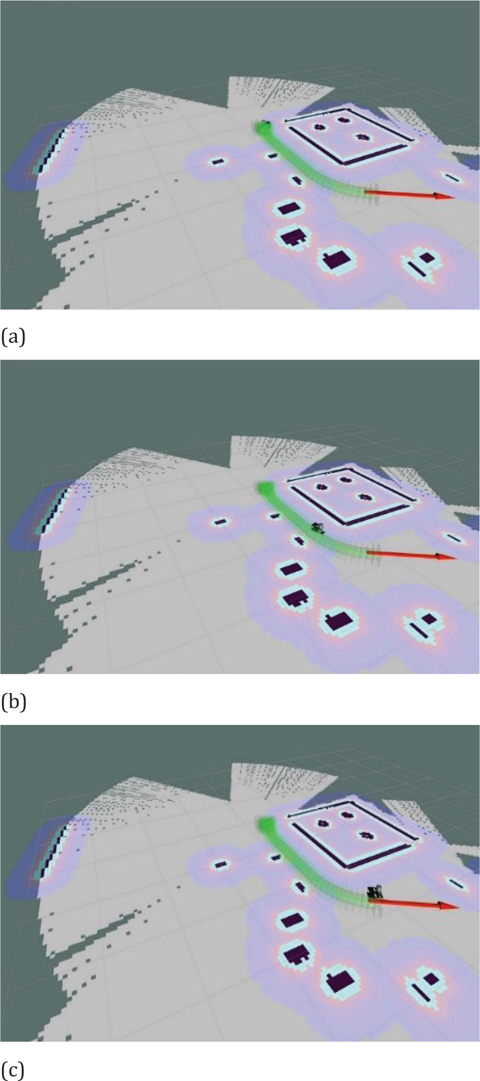
Figure 4.
Path planning with Hybrid A* node
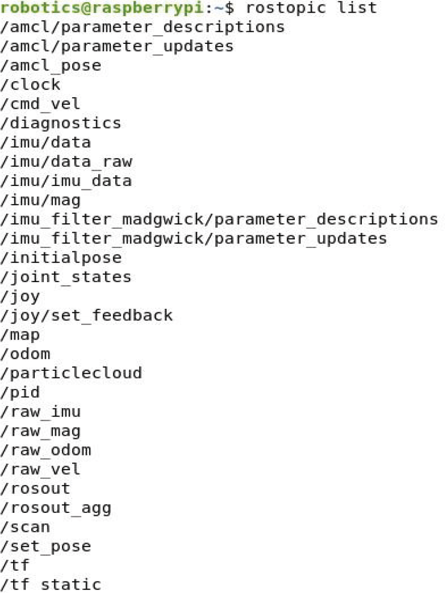
Figure 5.
Published and subscribed topics during localization process
Table 3.
Results of analytical calculations for each wheel of mobile transportation robot
| Slope Angle | Payload and System Mass (kg) | Tractional Force (Ftr) (N) | Total Driving (Fdrv) (N) | Tractional Torque (Tr) (Nm) |
|---|---|---|---|---|
| 0.0° | 130 | 318.83 | 19.38 | 15.34 |
| 2.5° | 130 | 318.52 | 33.28 | 15.32 |
| 5.0° | 130 | 317.61 | 47.16 | 15.28 |
| 7.5° | 130 | 316.10 | 60.99 | 15.20 |
| 10.0° | 130 | 313.98 | 74.74 | 15.10 |
| 12.5° | 130 | 311.27 | 88.38 | 14.97 |
| 15.0° | 130 | 307.96 | 101.89 | 14.81 |
| 17.5° | 130 | 304.07 | 115.25 | 14.63 |
| 20.0° | 130 | 299.60 | 128.42 | 14.41 |
Table 4.
Results of analytical calculations for each wheel of the mobile transportation robot
| Parameter | Mean | Std. Dev. | Min. | Max. | Range |
|---|---|---|---|---|---|
| Tractional Force (N) | 311.993 | 6.845 | 299.6 | 318.83 | 19.23 |
| Total Driving Force (N) | 74.388 | 37.38 | 19.38 | 128.42 | 109.04 |
| Tractional Torque (Nm) | 15.007 | 0.329 | 14.41 | 15.34 | 0.93 |
Table 5.
Comparison of implemented path planning algorithms
| Hybrid A* Algorithm | Move Base (A* Algorithm) |
|---|---|
| Shows strong performance in real-time path adjustments and obstacle avoidance.
|
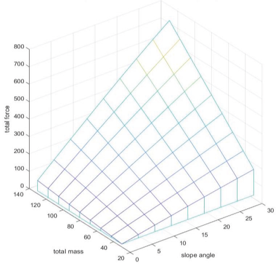
Figure 6.
The torque is changing in terms of mass and slope angle
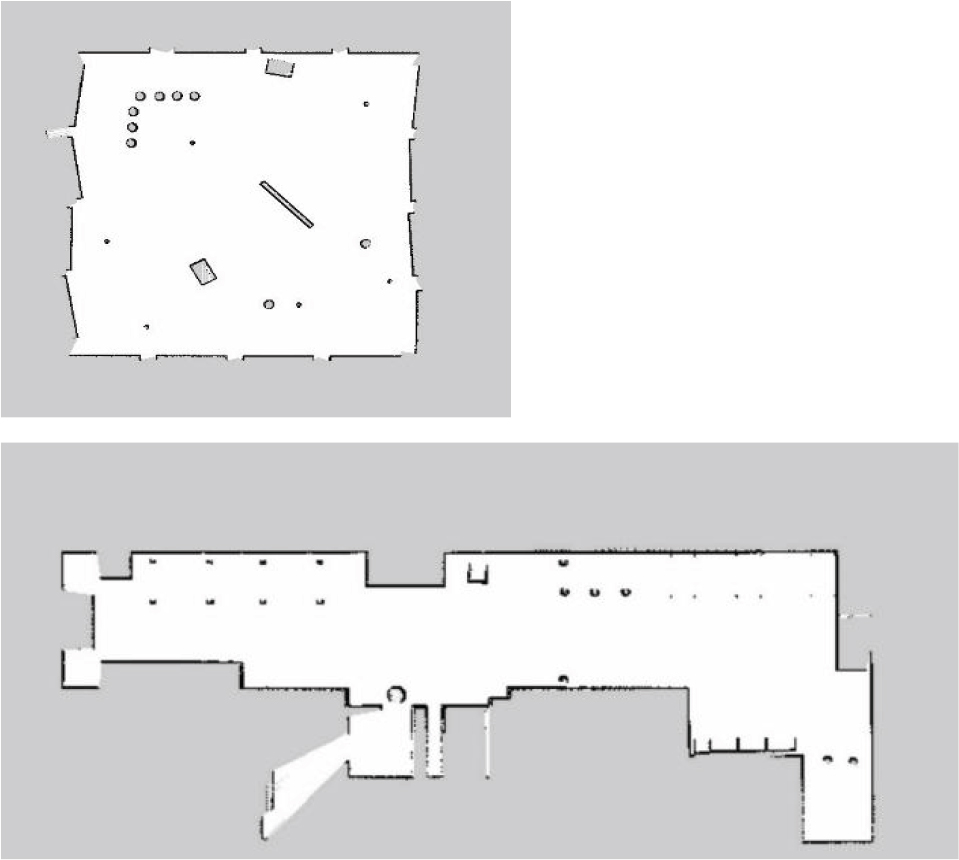
Figure 7.
Created maps by slam_gmapping node according to gazebo worlds on ROS
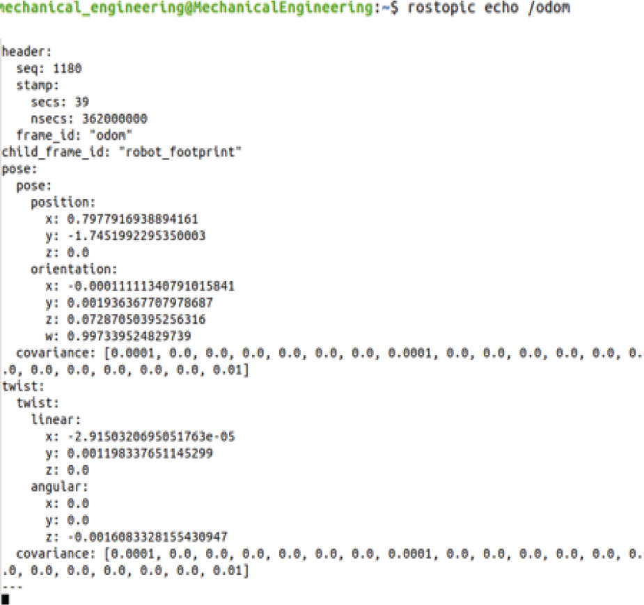
Figure 8.
Example output of the ROS odom topic obtained during experimental validation tests performed during the development phase of the AMR system generated during real-world AMR operation