

Wheeled Mobile Robot (WMR) refers to robots that navigate on the ground using motorized wheels to propel themselves. Among the branches of mobile robots, WMRs are simpler and more efficient than other designs, such as those that utilize grooves or legged robots. They are easy to design, produce, and program for linear and angular motion on a horizontal plane. This makes the WMRs an active field of research in order to fulfill the needs of surveys, patrols, emergency savings, identification, petrochemicals in automation, building structures, transportation, and healthcare. With numerous features, WMRs are being applied in various fields such as agriculture services and other industries [1–7]. Since then, the requirements for accurately controlling the movement trajectory of mobile robots with wheels have also increased.
Experiments show that between the two main types of WMR, nonholonomic robots are more difficult to control than holonomic robots [8]. Hence, this kind of system poses more problems for researchers.
The trajectory accuracy of holonomic robots is affected by various uncertain factors from the robot itself and external forces, making it more challenging to control the system [9].
To address these challenges, various solutions have been proposed to enhance the accuracy and trajectory tracking of nonholonomic wheeled mobile robots (WMRs) under uncertain interference factors. These solutions include fuzzy control [10–12], back-steppingbased control [13–15], and sliding mode control (SMC) [16–18], among others [5, 12, 19–21]. However, controllers based on the “no-slip wheel” hypothesis, such as SMC [16, 18, 22], adaptive control [23–26], and backstepping control [13, 14], fail to meet the system’s requirements for stability and precise trajectory tracking.
In recent years, several methods have been proposed to solve interference problems in WMR control. One of them is robust adaptive tracking control [26–28], a tracking controller that combines disturbance observer and a responsive compensation mechanism to deal with unstable systems. Therefore, the errors and responses are limited. In [29], the problem of trajectory tracking for WMR under conditions of system uncertainty and external disturbances was solved. By using a fuzzy logic system (FLS) for model estimation and an adaptive fuzzy observer for estimating unmeasured velocities, the position errors are minimized and system response is fast.
Wheel slips in WMR are also an interesting problem for many researchers. In order to overcome the challenges in a conventional backstepping controller, a dynamic surface controller (DSC) is developed [5, 30], which incorporates skidding and sliding mechanisms. In [17], a control scheme combining sliding mode control with a backstepping observer is proposed for WMRs with unknown sliding and model uncertainty. This algorithm mitigates the effects of system uncertainties, disturbances, and vibrations inherent in sliding mode control; however, the illustrative results are not satisfactory. A control technique utilizing a fuzzy PID controller, combined with IMU and feedback current, is introduced in [31] to reduce slippage caused by environmental factors. While the results indicate that this control scheme is effective, system stability is not addressed. In [17, 32], a controller based on a disturbance observer that accounts for skidding and sliding is presented, however the error in this algorithm remains significantly high.
The robust adaptive controller developed in [33] accounts for disturbances and wheel slips, with the WMR dynamics explicitly considering wheel slip in the tracking controller’s design. A disturbance observer is utilized to estimate robot uncertainties and slip. However, the controller has only been verified through simulations, and the discontinuous transition in the control law may lead to instability.
This paper aims to deal with the shortcomings of the approach presented in [33] for tracking control of Wheeled Mobile Robots (WMRs). The proposed control scheme consists of two loops: an inner loop, which uses a PID controller for precise wheel speed regulation, and an outer loop, which employs a disturbance observer to accurately track the reference trajectory in case of disturbances and uncertainties. The key contributions of this paper are as follows:
Improvement of [33]: The outer loop tracking controller is re-derived using Lyapunov stability theory, and a novel method for handling noninvertible matrices is introduced.
Simulation Validation: The proposed control structure is thoroughly tested in simulations, demonstrating significant improvements in system response compared to the method in [33].
Experimental Verification: The effectiveness of the proposed scheme is further validated through realworld experiments on a WMR, with the results confirming its superior performance.
In this research, the WMR model is referred from [33], the kinematics and dynamics model of WMR, which takes account of wheel slips, and is summarized as follows:
The robot parameters are defined and shown in Fig. 1. In which, G (xG, yG) is the center of mass of the WMR platform, M (xM, yM) is the midpoint of the driving wheels, D (xD, yD) is the desired position; θ is the orientation of WMR; 2b is the width of WMR; r is the wheel radius; ep1, ep2 are the position errors between M and D in the MXY coordinate; a is the distance between M and G; γR,γL are longitudinal slip factors of the right and left driving wheels, respectively; η is the lateral slip factor along the wheel shaft; I, B, Q, C and G are weighting matrices and vectors in WMR dynamic, which are defined in details in [33]:
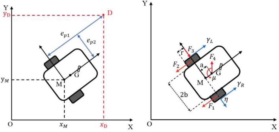
WMR in coordinates and its dynamic factors
Similar to the approach in [33], the control scheme for the WMR consists of two loops arranged as a cascade control system, as shown in Fig. 2. The outer loop is responsible for controlling the robot’s position. This controller incorporates a disturbance observer to compensate for disturbances, system uncertainties, and model errors. Meanwhile, the inner loop manages wheel speed control, ensuring that the wheels follow the speed commands generated by the outer loop.
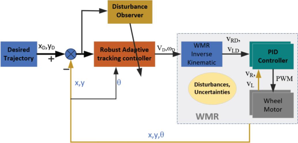
Overall structure of proposed control scheme
The PID controller, known for its wide application due to its stability, robustness, and reliable control performance, is used in the inner loop. As a result, the overall control system heavily depends on the effectiveness of the outer loop controller. Therefore, this section focuses on the outer loop controller and the integration of the disturbance observer to enhance system performance.
In the MXY coordinate, the errors between the robot position M (xM, yM) and its desired point D (xD, yD) are determined as:
Taking derivative of (4) with respect to time, it can be obtained as [33]:
Then, the objective of the WMR control is to find the control rule for v so that ep converges to zero.
When the WMR follows the reference, the position errors along x and y directions converge to zero. Hence, to find the control rule for position controller, the Lyapunov candidate function is chosen as:
From (6), it can be obtained:
From (11), the control law v is selected as:
Then (11) becomes:
Thus, the system is asymptotic stable with the control law in (12) and ep converges to zero in term of Lyapunov stable criteria.
From (11), the term d(.) is an unknown factor, thus the control signal cannot be calculated directly. In this research the disturbance observer in [34] is employed to estimate this term.
Consider the system (6), the disturbance observer [34] is designed as:
The disturbance estimation error is defined as:
Then the derivative of this error can be determined as:
From (14) and (16), it is easy to obtain:
It is assumed that the disturbance is low variation, then
With the disturbance observer in (14), the control signal in (12) will become:
Then the equation (6) will become:
Then the derivative of this function will be:
If λ and L are chosen as λ > 1/2 and L > 1/2, then
In (7), when
Hence h(.) is not invertible, the calculation of the control signal v cannot be implemented. To resolve that problem, instead of using law as [33] in this research, the value of ep1 in (7) is introduced to be replaced by
The detail diagram of the tracking controller with disturbance observer is depicted in Fig. 3.
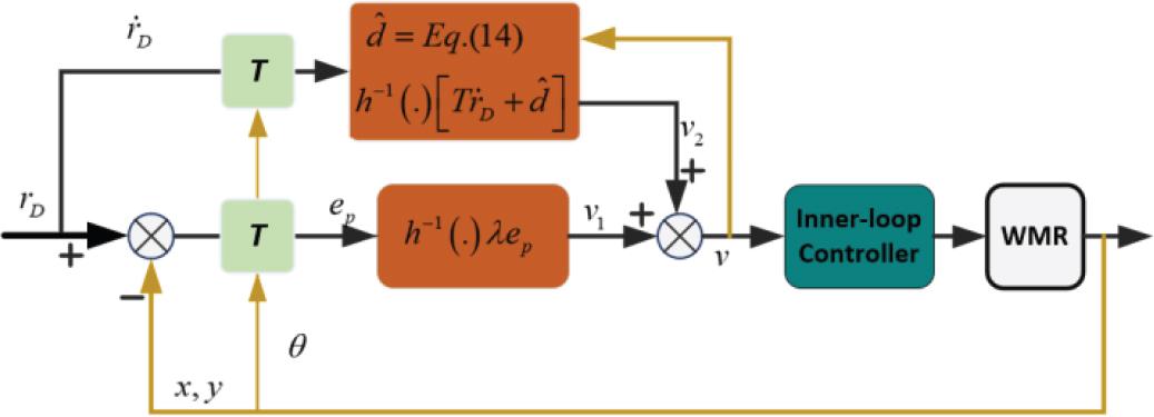
Diagram of outer-loop tracking controller
The block diagram for a WMR experimental control setup is shown in Fig. 4. In this setup, the outer loop controller is executed on the embedded computer. In which, the WMR position and orientation is determined by an ArUco marker and vision method. Based on these measurements, the adaptive controller with disturbance observer described in (19) is implemented to find the reference signals for the inner loop controller. The inner loop controller is executed on the microcontroller to control the rotational speed of the right and left driving wheel of robot.
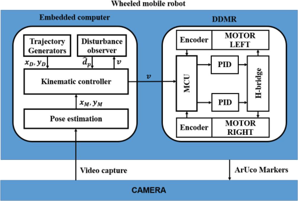
Block diagram of WMR experimental control implementation
The apparatus of WMR hardware, components and experimental control setup are shown in Fig. 5 to Fig. 7. In this setup, the IP camera is mounted on the top position so that it can cover the robot and its experimental trajectory. The robot position and orientation is detected by the ArUco marker that is placed at midpoint of driving wheels M.
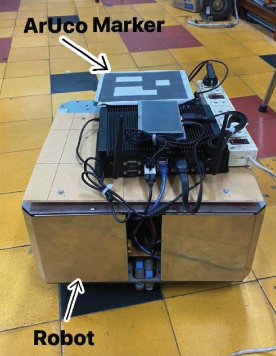
Apparatus of WMR with an ArUco marker and embedded computer
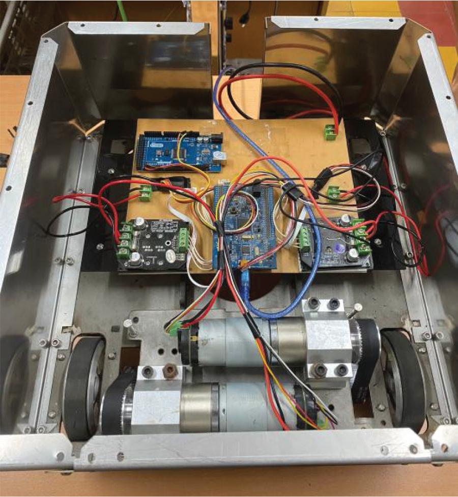
Setup of electric components in WMR
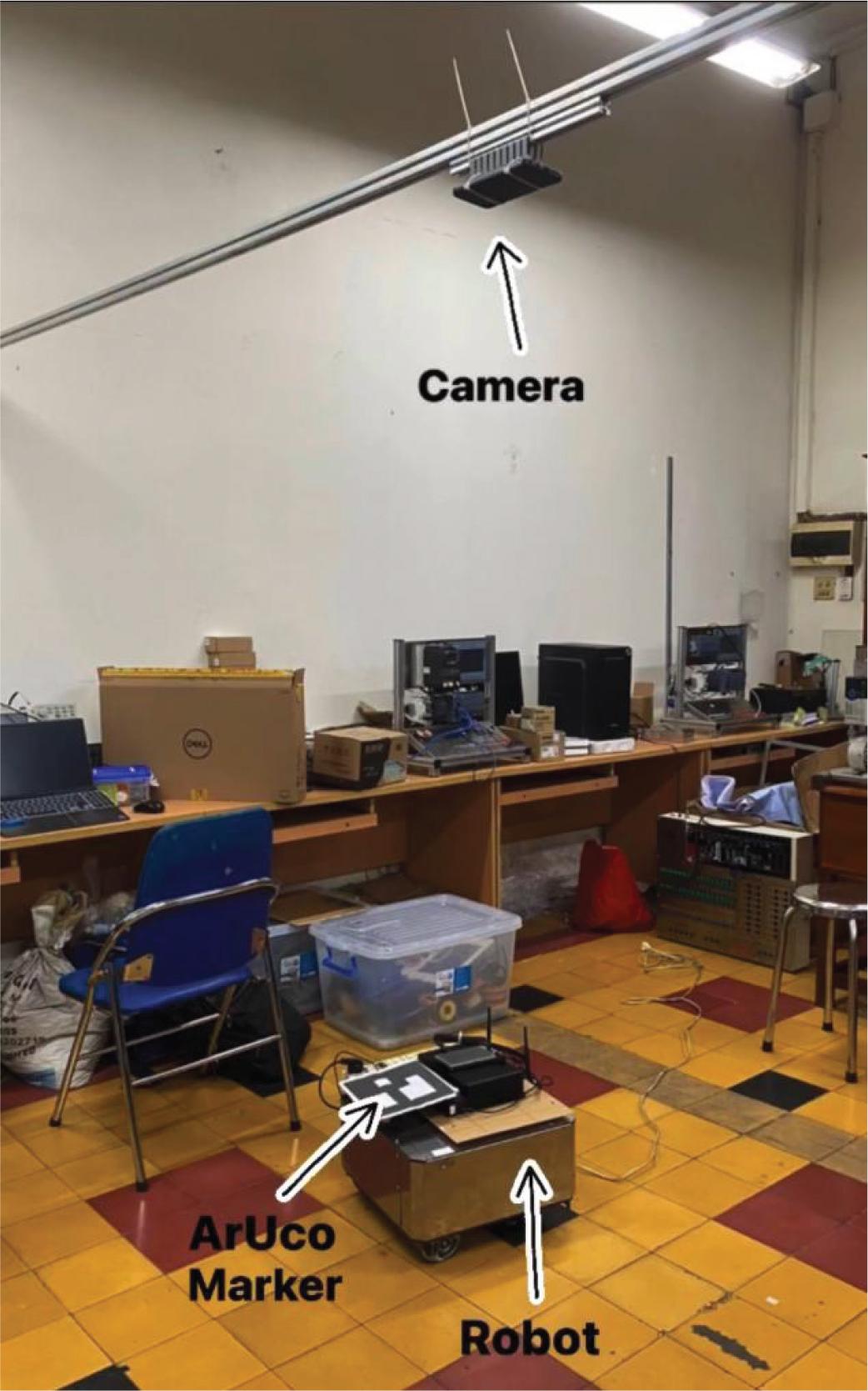
Overall image of experimental control setup
The experimental procedure involves the following steps:
- (1)
Deploy the PID controller for the robot’s inner loop on the microcontroller.
- (2)
Set up the mounting frame for the IP camera and perform calibration using a checkerboard pattern.
- (3)
Deploy the pose estimation program on the embedded computer to gather position data (x, y, 0) from the camera.
- (4)
Deploy the adaptive controller with a disturbance observer on the embedded computer.
- (5)
Position the robot at its initial point for trajectory tracking.
- (6)
Execute the programs through ROS.
- (7)
Collect the data and print the results.
- (8)
Stop the observation process by terminating the program.
To evaluate the proposed controller, it was tested in both simulation and experimental settings.
In the simulation, the WMR model and the proposed controller were implemented in MATLAB Simulink. Two trajectory cases were used to verify the simulation results: an eight-shaped trajectory and a circular trajectory. The mathematical expression for the eightshaped trajectory is presented in Equation (23), while the circular trajectory is described in
Equation (24):
The simulation parameters for the WMR are set in the condition of our experiment robot as Table 1; and 20 the controller parameters are set as
Robot simulation parameters
| Parameter | Description | Value |
|---|---|---|
| r | Wheel radius (m) | 0.06 |
| 2b | Driving wheel distances (m) | 0.31 |
| mG | Weight of robot flatform (kg) | 10 |
| mW | Weight of robot wheel (kg) | 0.7 |
| Distance of MG (m) | 0.1 | |
| IG | inertial moment of the platform about the vertical axis through point G (kg.m2) | 0.2 |
| Iw | inertial moment of each wheel about its rotational axis (kg.m2) | 0.0013 |
| ID | inertial moment of each wheel about its diameter axis (kg.m2) | 0.0038 |
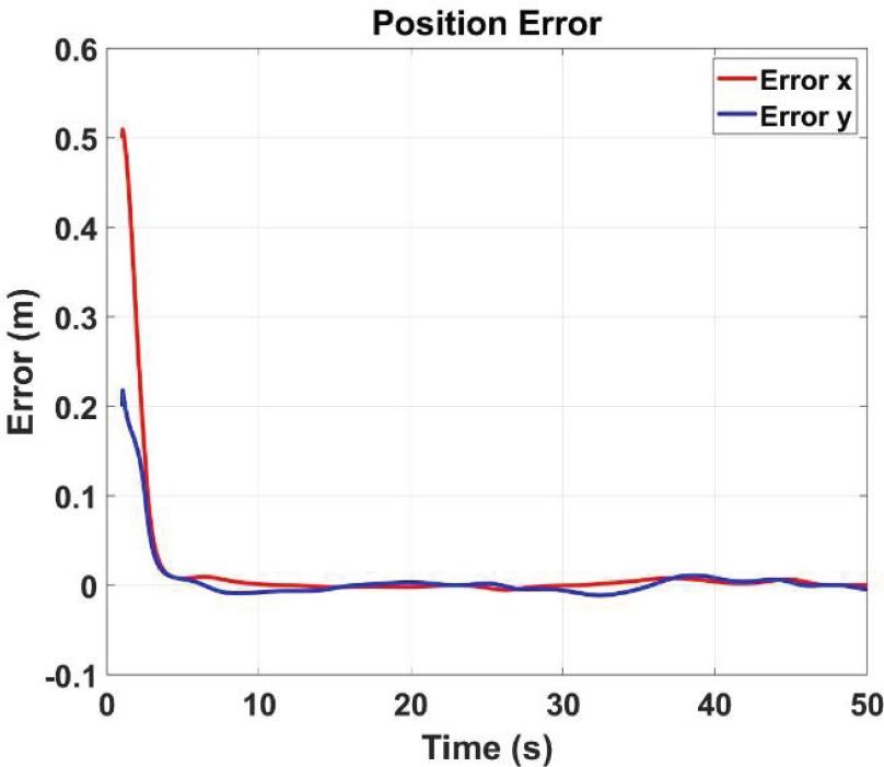
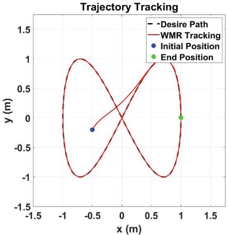
Simulation results are presented in Fig. 8 through Fig. 23, demonstrating the performance of the proposed controller on circular and eight-like trajectories. Additionally, the algorithm from [33] is evaluated for comparison with the proposed controller. The simulation results indicate that both controllers can effectively track the reference trajectories. Tracking errors for both controllers are shown in Fig. 9, Fig. 13, Fig. 17 and Fig. 21.
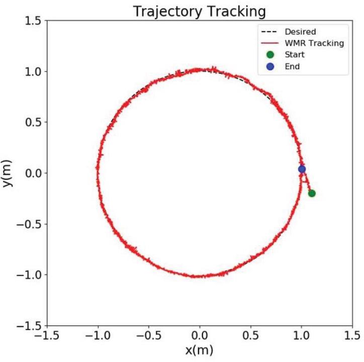
Circular trajectory tracking result by using proposed controller
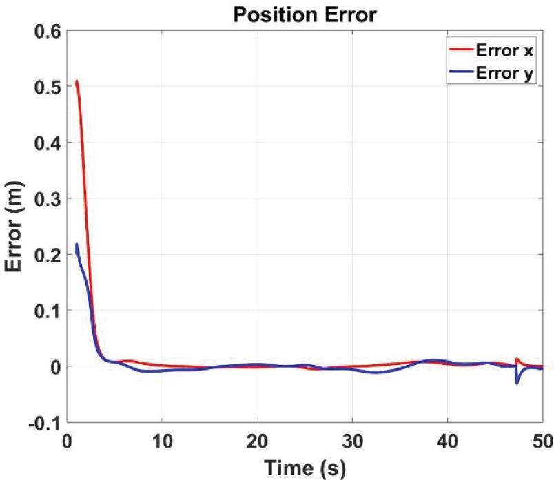
Circular trajectory tracking errors by using proposed controller
It is evident that the tracking errors in Fig. 9 and Fig. 17 converge smoothly to small values, while the controller from [33] exhibits significant sudden changes when the error is small, as shown in Fig. 13 and Fig. 21. This behavior is due to the discontinuous translation in the matrix h(.) when ep → 0 in equation (19) changes.
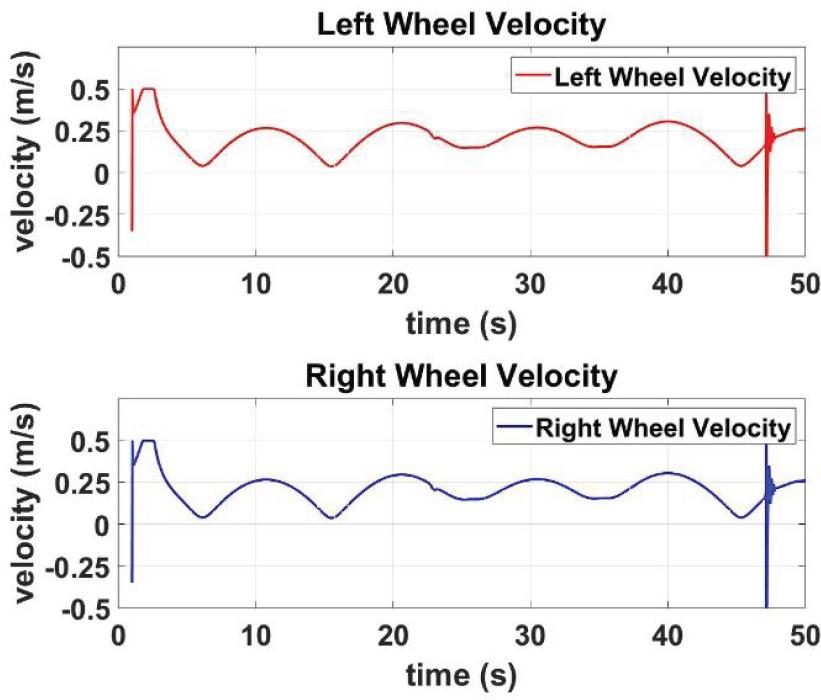
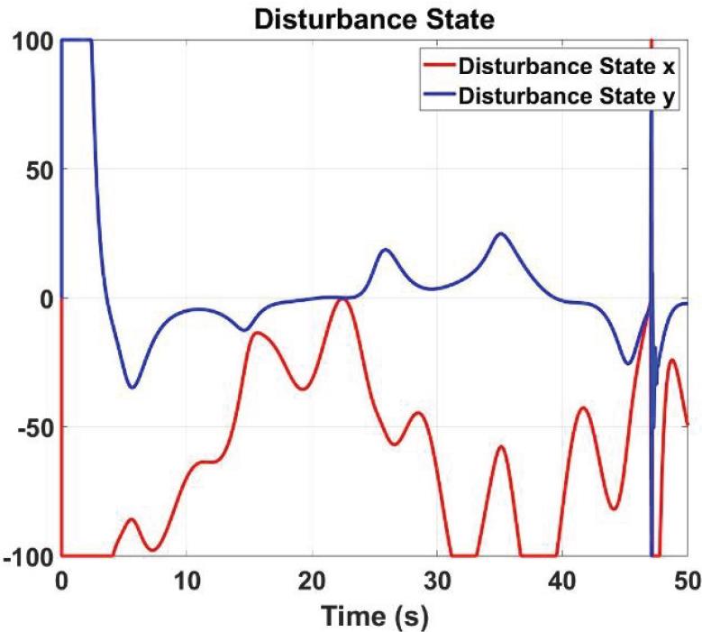
The proposed controller’s significant advantages over the one in [33] are evident in the wheel speed control signals (Fig. 10, Fig. 14, Fig. 18, and Fig. 22) and disturbance estimation results (Fig. 11, Fig. 15, Fig. 19 and Fig. 23).
Reference speeds of driving wheels with respect to circular trajectory generated by proposed controller
Disturbances estimation with respect to circular trajectory from proposed controller
It can be observed that the wheel velocities and estimated disturbances are stable and smooth with the proposed controller, whereas the controller in [33] exhibits large variations, particularly from the 47th second onward, as seen in Fig. 15, and Fig. 23. These variations may lead to system instability.
The simulation results confirm that the proposed controller performs effectively, exhibiting accurate-tracking, smooth responses, precise estimations, and overall system stability.
Circular trajectory tracking result by controller from [33]
Circular trajectory tracking error by controller from reference [33]
Following the successful simulations, the proposed controller was implemented and tested under real-world conditions using a physical robot. In this experimental setup, the robot was tasked with tracking circular and square trajectories, both under noload and 5 kg load conditions.
Reference speeds of driving wheels with respect to circular trajectory generated by controller from [33]
Disturbances estimation by controller from [33]
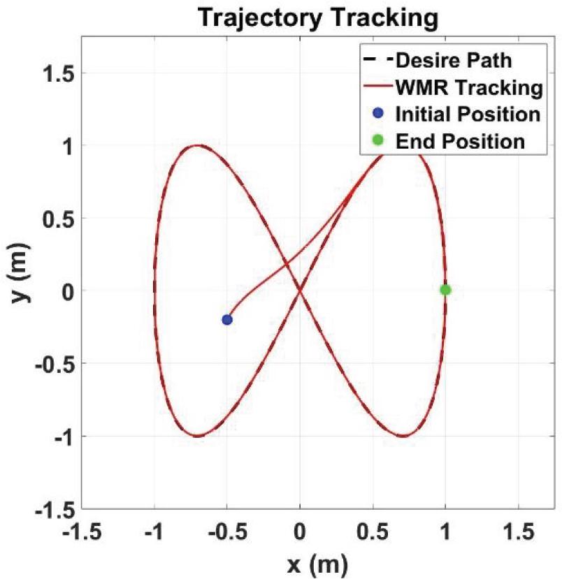
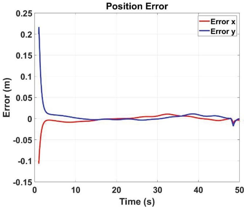
Eight-like trajectory tracking result by using proposed controller
Eight-like trajectory tracking error with respect to eight-like by proposed controller
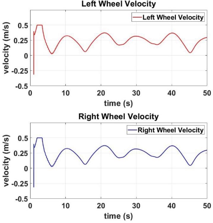
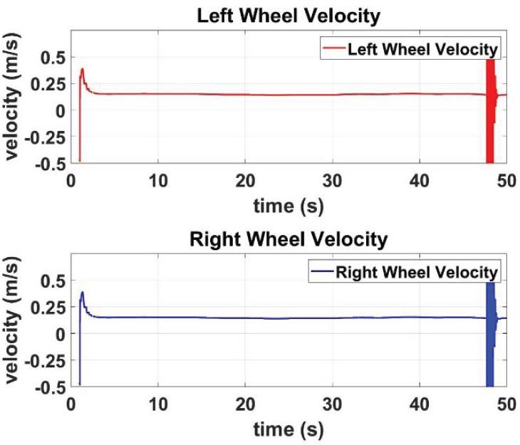
Reference speeds of driving wheels with respect to eight-like trajectory generated by proposed controller
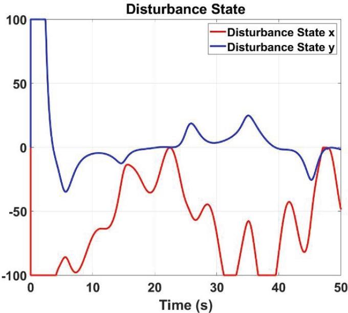
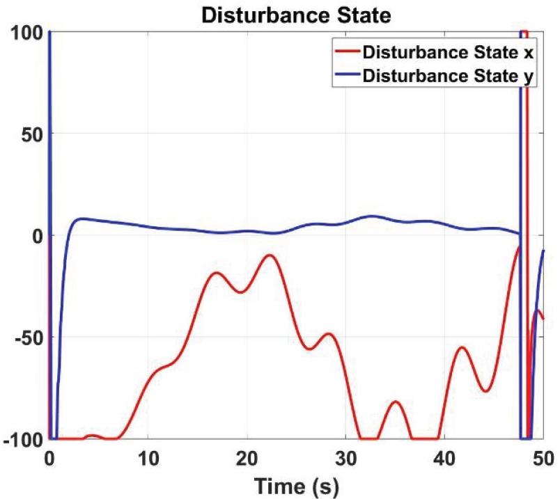
Disturbances estimation with respect to eight-like trajectory from proposed controller
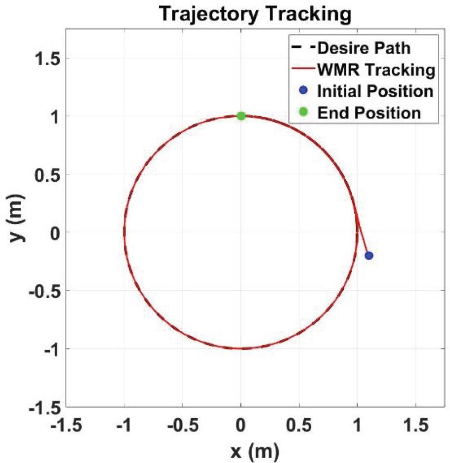
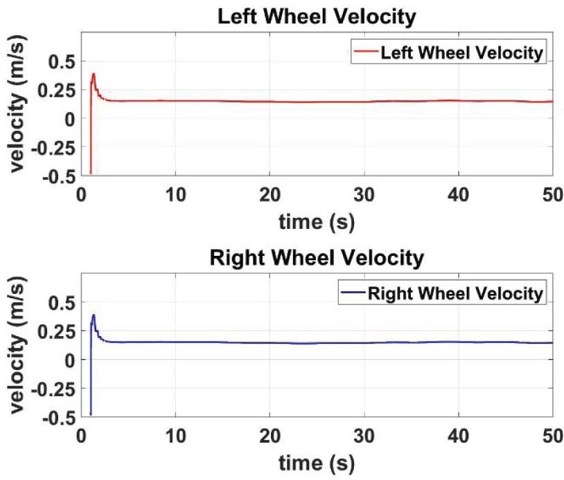
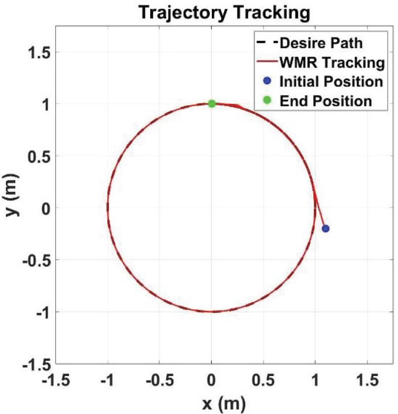
Fig. 24 through Fig. 27 present the control results obtained from the real-world experiments. The results demonstrate that the controller successfully guides the robot along the circular trajectory (Fig. 24) with a small steady-state error of less than 3 cm (Fig. 25). The controller’s output signals, represented by the wheel velocities, are shown in Fig. 26. For the circular trajectory, the right wheel appears to maintain a constant speed of 0.06 m/s, while the left wheel speed adjusts to follow the trajectory with smaller speed.
Eight-like trajectory tracking result by controller from [33]
Eight-like trajectory tracking error by controller from reference [33]
Reference speeds of driving wheels with respect to Eight-like trajectory generated by controller from [33]
Disturbances estimation with respect to eight-like by controller from [33]
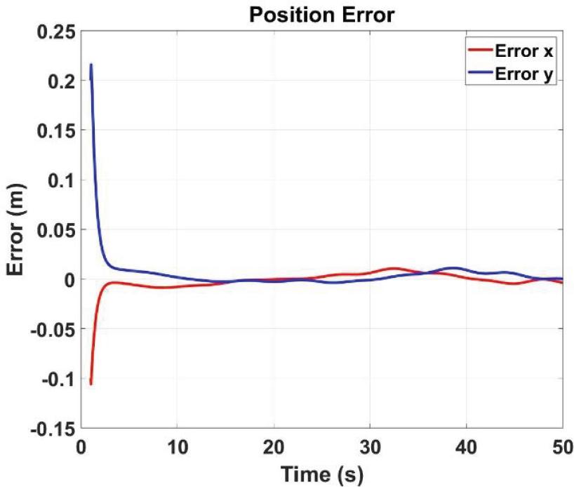
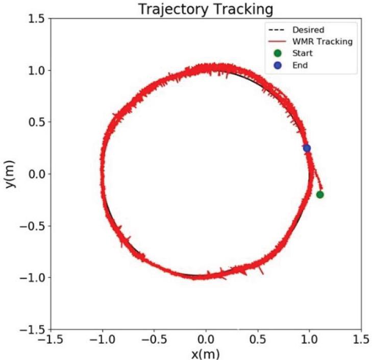
Experimental tracking result with respect to circular trajectory
Experimental tracking errors with respect to circular trajectory
Experimental wheels velocity with respect to circular trajectory
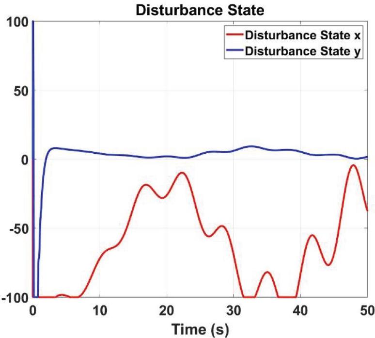
Experimental disturbances estimation with respect to circular trajectory
The disturbance estimation results are illustrated in Fig. 27.
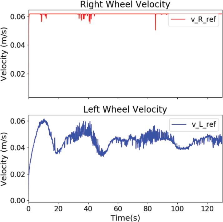
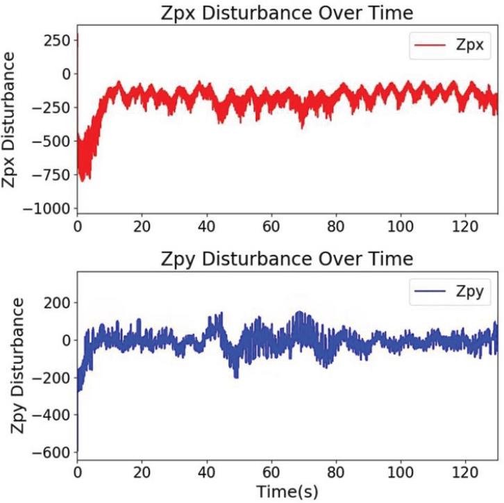
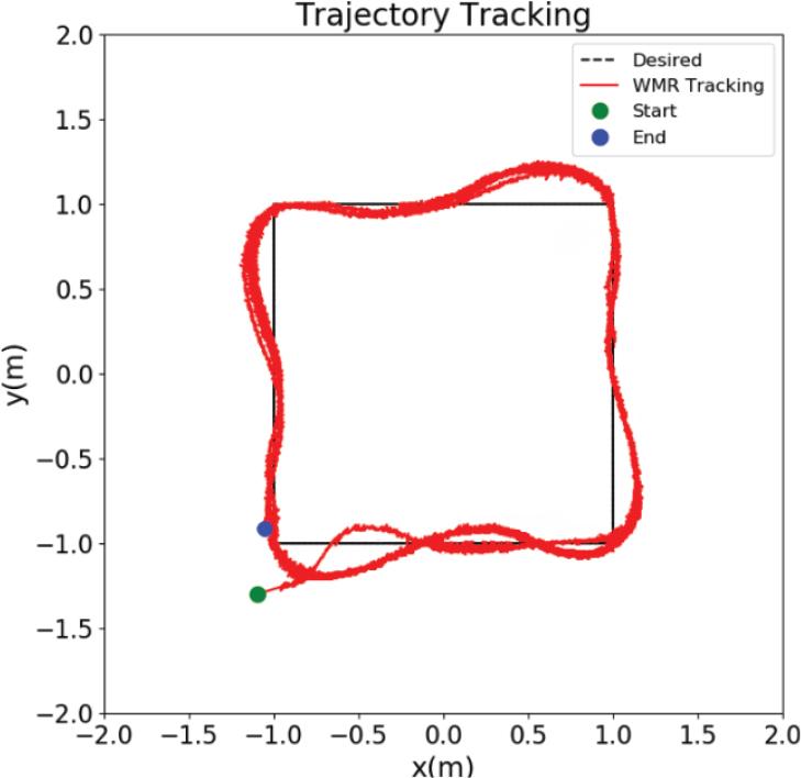
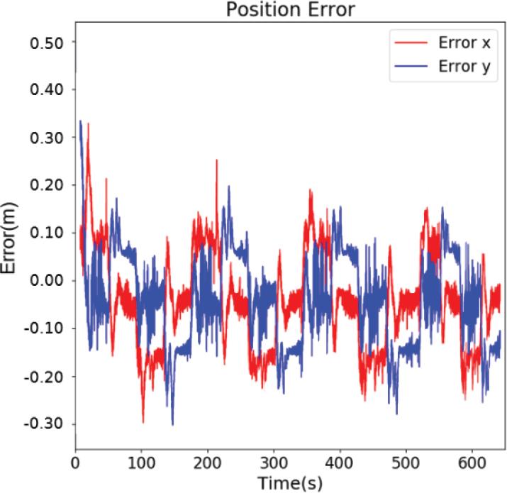
Similarly, the control results for the square trajectory are shown in Fig. 28 through Fig. 31. Fig. 28 illustrates the tracking performance for the square trajectory. It can be observed that there is an overshoot when the reference changes its orientation, which occurs due to the robot’s inertia and reference speed, causing it to continue moving forward until it adapts to the new orientation. Fig. 30 depicts the wheel speeds, showing that the left wheel speed decreases rapidly to accommodate the sudden change in the reference trajectory. The disturbance estimation results are presented in Fig. 31.
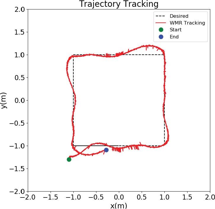
Experimental tracking result with respect to square trajectory
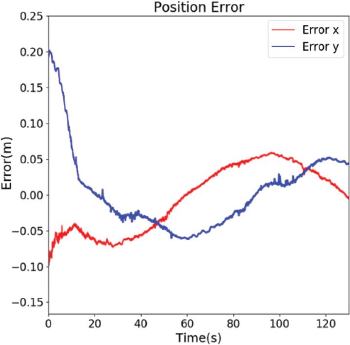
Experimental tracking error with respect to square trajectory
Experimental wheels velocity with respect to square trajectory
Experimental disturbances estimation with respect to square trajectory
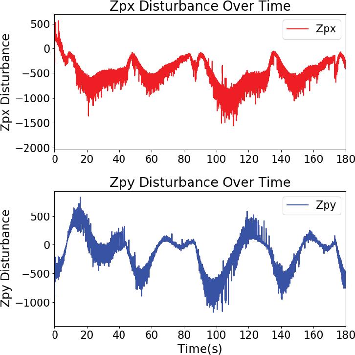
Finally, the controller is verified in long-time and load conditions. In this test, the robot carries a 5 kg load and track to circular and square trajectories in 4-loops. The tracking results are shown in Fig. 32 and Fig. 35. It can be seen that the controller successfully adapts to varying load conditions. Furthermore, the control performances are kept stable in all loops, this demonstrates that the controller is stable and robust over time. The control signals with respect to trajectories, are displayed in Fig. 34 and Fig. 37. They show that the wheels’ speeds are similar after each cycle. This proves the robustness and stability of the controller.
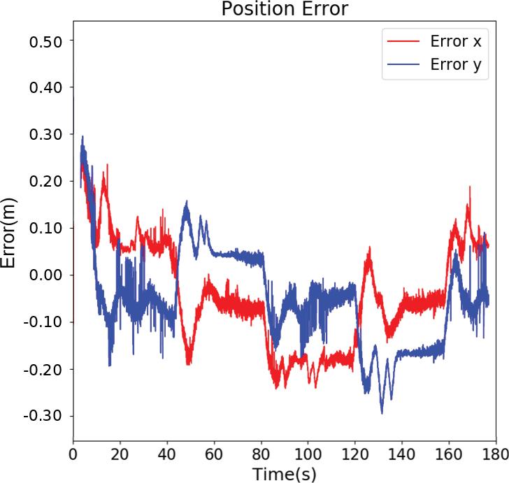
Experimental tracking result with respect to 4loops circular trajectory under 5 kg load
Experimental tracking errors with respect to 4loops circular trajectory under 5 kg load
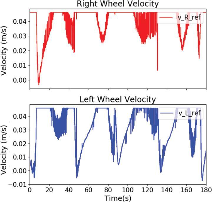
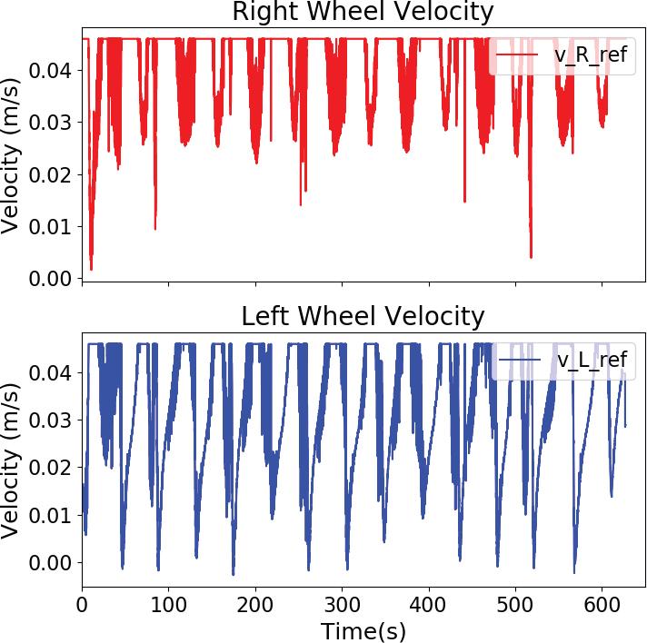
Experimental wheels velocity with respect to 4loops circular trajectory under 5 kg load
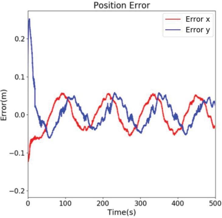
Experimental tracking result with respect to 4loops square trajectory under 5 kg load
Experimental tracking errors with respect to 4loops square trajectory under 5 kg load
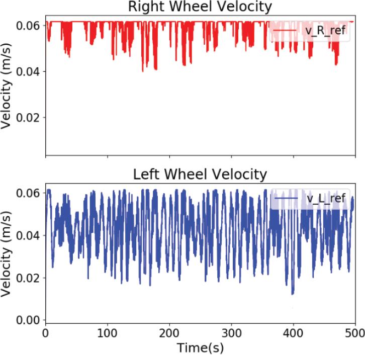
Experimental wheels velocity with respect to 4loops circular trajectory under 5 kg load
Finally, the proposed controller is tested under longduration and load conditions. In this experiment, the robot carried a 5 kg load while tracking circular and square trajectories over four loops. The tracking results are shown in Fig. 32 and Fig. 35. The results indicate that the controller adapts well under load conditions, maintaining stable control performance throughout all loops. This demonstrates the controller’s stability and robustness over time. Furthermore, the control signals corresponding to the trajectories are displayed in Fig. 33 and Fig. 35, showing that the wheel speeds remain consistent after each cycle. This consistency further proves the robustness and stability of the controller.
In this research, a robust adaptive controller with a disturbance observer was investigated for nonholonomic robots, based on the kinematic and dynamic models of Wheeled Mobile Robots (WMRs). The disturbance observer was employed to handle system uncertainties and external disturbances. The stability of the proposed controller was proven using both Hurwitz and Lyapunov stability criteria.
The study primarily focuses on the outer loop tracking control scheme, which improves the performance of a previously proposed method by incorporating a disturbance handler and addressing remaining issues, such as providing a clear mathematical interpretation for non-invertible matrices and implementing this directly.
Moreover, extensive simulations and experimental results were conducted, demonstrating the proposed controller’s efficiency, robustness, and stability.