

The rapid advancement of imaging sensors over recent decades has paved the way for a plethora of intelligent perception algorithms [1, 2]. Leveraging these capabilities, vision technology has made significant strides in various fields, including space robotics [3], robot manufacturing, rapid object detection, and tracking. Industrial Robot Vision (IRV), which integrates computer vision into industrial manufacturing processes, presents a nuanced approach compared to traditional computer vision methodologies. Typically, robot vision systems prioritize tasks such as harvesting [4], human-robot interaction [5], and robot navigation [6]. These systems find application across a spectrum of areas, including complex system part identification, defect inspection, Optical Character Recognition (OCR) reading, 2D code reading, piece counting, and dimensional measurement [7]. Figure 1 illustrates a typical industrial robot vision system configuration, comprising fundamental components such as cameras and control systems (e.g., Robots, PLCs). Additional features like illumination, user interaction, data storage, and remote control are gradually integrated to improve system efficiency Object images captured are typically subjected to pre-processing, segmentation, and feature extraction on a server. Controlled lighting conditions and fixed camera positions ensure the prominence of critical features, while the control system receives task execution instructions from the server.
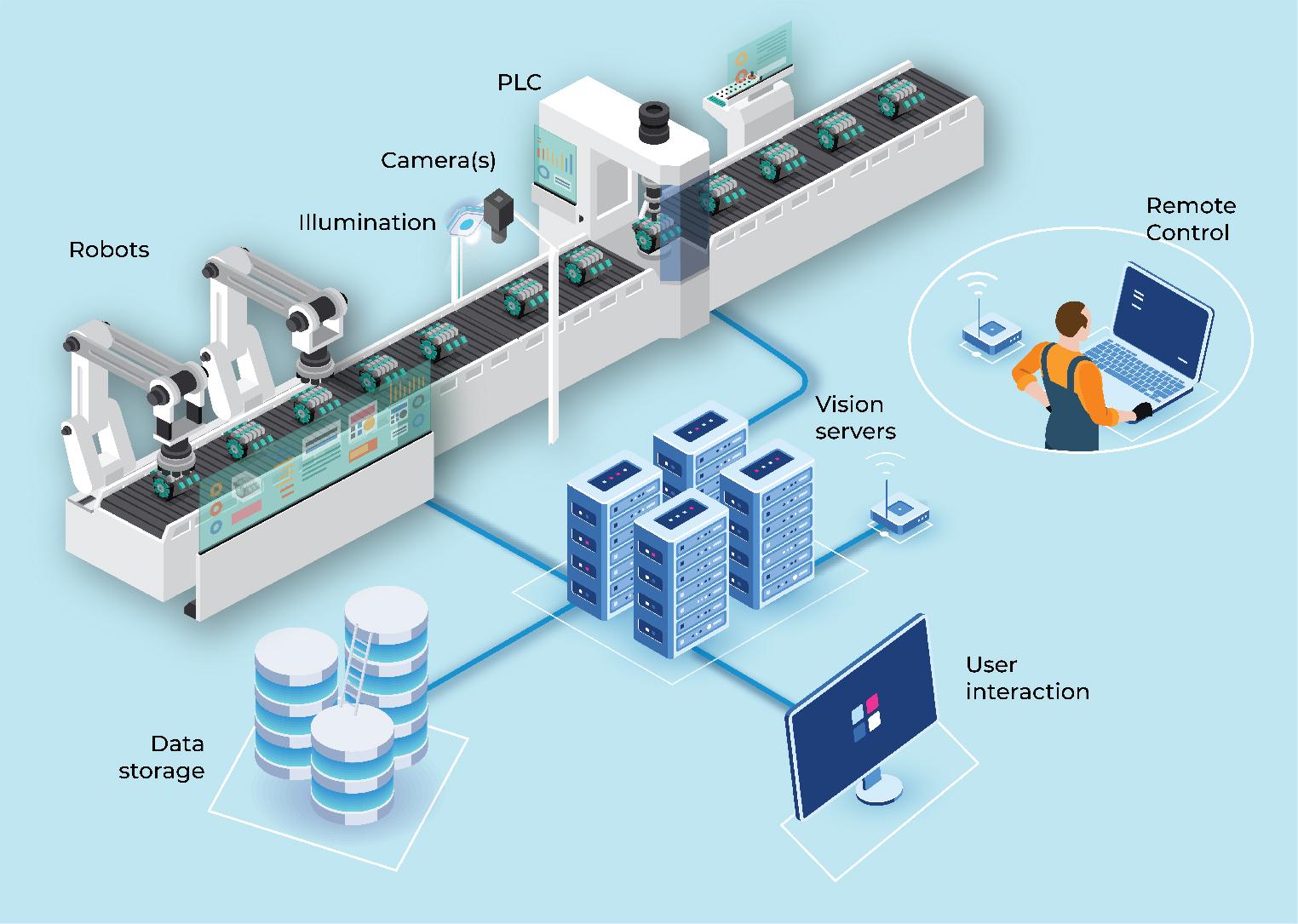
Overview of the industrial robot vision system
Camera calibration is indispensable in robot vision systems to ensure precise object location and accurate measurements [8]. However, the process is highly susceptible to environmental changes, encompassing variations in lighting, temperature, and humidity, potentially introducing inaccuracies by impacting intrinsic and extrinsic parameters. Despite efforts to precisely estimate camera parameters, real-world complexities such as lens distortions and non-linearities may not be fully accounted for, leading to calibration inaccuracies. Notably, challenges arise when the object is not directly under the camera, resulting in an incorrect prediction of the object’s center relative to the reference point. To mitigate these challenges, two primary approaches are considered: i) optimization of intrinsic parameters and ii) recognition of 3D objects to estimate the center point. Numerous algorithms have been developed to obtain intrinsic parameters for imaging sensors [9–11]. Intrinsic calibration typically involves a camera that observes anchor points in a calibration pattern, with commonly used patterns including checkerboards [12], coplanar circles [13, 14], and AprilTags [15]. Traditional calibration methods, such as those supported by OpenCV [16] and MATLAB [17], have become commonplace, leveraging the advantage of calibration toolboxes. However, deploying these approaches in factory settings proves challenging, as they are susceptible to noise and artifacts that can degrade calibration performance.
For industrial vision systems, several techniques for 2D camera calibration have been introduced to achieve precise object localization. Brown’s Plumb Line method [18], an early notable approach, addresses the lens asymmetry issues encountered during manufacturing. This method requires the determination of 10 parameters and achieves high accuracy, with deviations as low as ±0.5mm a distance of 2m.
Innovations by Clarke, Fryer and Chen [19] have adapted this method to use with CCD sensors, enhancing efficiency. Lu and Chuang [20] utilized a flat monitor on which they drew lines and then estimated the projection between the image plane and the monitor plane through multiple shots to calibrate the camera. The Two-Stage method [21–23] focuses on real-time calibration using black squares on a white background, achieving uncertainties around ±1mm at 2m Direct Linear Transformation (DLT)-based methods [24–27] simplify calibration models and have been widely adopted. However, these approaches tend to fail in the case of localizing 3D-shaped objects. Due to their 3D natural shape, the locations determined by these calibration methods are the locations of their projections on the image rather than their true spatial positions. Consequently, the error distance to the real location of the objects remains significant. Zhang’s technique [28], requiring only a planar pattern, offers flexibility with quicker application in industrial contexts, albeit with slightly higher uncertainties. Beyond these, researchers have tailored calibration methods for specific applications, such as high-speed tensile testing machines and unmanned vehicle guidance, providing unique insights and experimental results. However, these approaches tend to fail in the case of localizing 3D-shaped objects. Building upon foundational studies such as Siddique et al. [29], who explored 3D object localization using 2D estimates for computer vision applications, our work seeks to advance these concepts by integrating more sophisticated calibration methods and deep learning techniques for improved accuracy and efficiency in industrial settings.
Due to their 3D natural shape, the location determined by calibration methods is in fact the location of their projections on the image instead of their real location. Therefore, the error distance to the real location of the objects still remains. In addition, Xiem HoangVan and Nam Do [30] introduced a machine learning – regression-based method for improving the accuracy of 3D object localization. Our method is created based on mathematical modeling of 3D objects and their projected image in the 2D plane and is followed by a regression-based algorithm to achieve model parameters.
In this paper, we proposed a novel approach (MCalib) with the following contributions:
- 1)
We validated the proposed work in rigorous experiments using a checkerboard. The results show that our approach outperforms the previous in estimation accuracy.
- 2)
We propose an efficient 3D localization method designed to accurately calculate the translation vector between the calibration center target and the initialized center point with sub-pixel localization accuracy. This method demonstrates robustness to noise, ensuring reliable performance in various conditions.
- 3)
We provide the source code of M-Calib to the research community, offering an easy-to-use calibration toolbox specifically tailored for monocular cameras. This resource is openly accessible at: https://github.com/NguyenCanhThanh/MonoCalibNet, facilitating further research and application development in the field.
The remainder of this paper is organized as follows: Section 2 delves into the intricacies of the problem statement, offering a comprehensive understanding of the challenges at hand.
We unveil our novel method for isometric flat 3D object localization, elucidating the deep learning methodologies employed and elucidating the procedural steps in Section 3. Section 4 presents the experimental setup and evaluates the performance of our proposed method using relevant metrics. Finally, Section 5 concludes the paper, summarizing the key findings, discussing potential future research directions, and emphasizing the significance of our contributions.
The problem addressed in this study lies at the intersection of machine vision and 3D object localization within industrial robot vision systems. While conventional 2D camera calibration methods, such as Brown’s Plumb Line Method and Tsai’s Two-Stage Method, have proven effective for achieving high accuracy in object localization, their limitations become evident when confronted with 3D-shaped objects. The inherent challenge arises from the fact that these methods determine object locations based on their projections onto the 2D image plane, resulting in inaccuracies in representing the true 3D positions. This discrepancy is especially pronounced in industrial contexts where precise object localization is crucial for tasks such as robotic automation, and quality control. Figure 2 illustrates the challenges when estimating the center of 3D objects. Under the influence of optical projection, the initial estimated center position (green point) often tends to deviate from the actual center (red point) position. To address this gap, we propose a novel approach, M-Calib, leveraging efficient 3D localization techniques to overcome the limitations of traditional 2D calibration methods. The objective is to enhance accuracy, particularly in the localization of isometric flat 3D objects, thereby contributing to the advancement of machine vision applications in industrial environments.
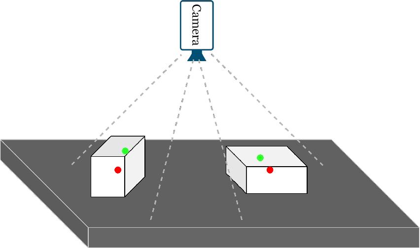
Illustration of industrial robot vision system: the green point is the initialized estimate center point, and the red point is the actual center point
Figure 3 presents a visual representation of our proposed calibration methodology, centered around the deliberate choice of a checkerboard as the calibration pattern for two significant reasons.
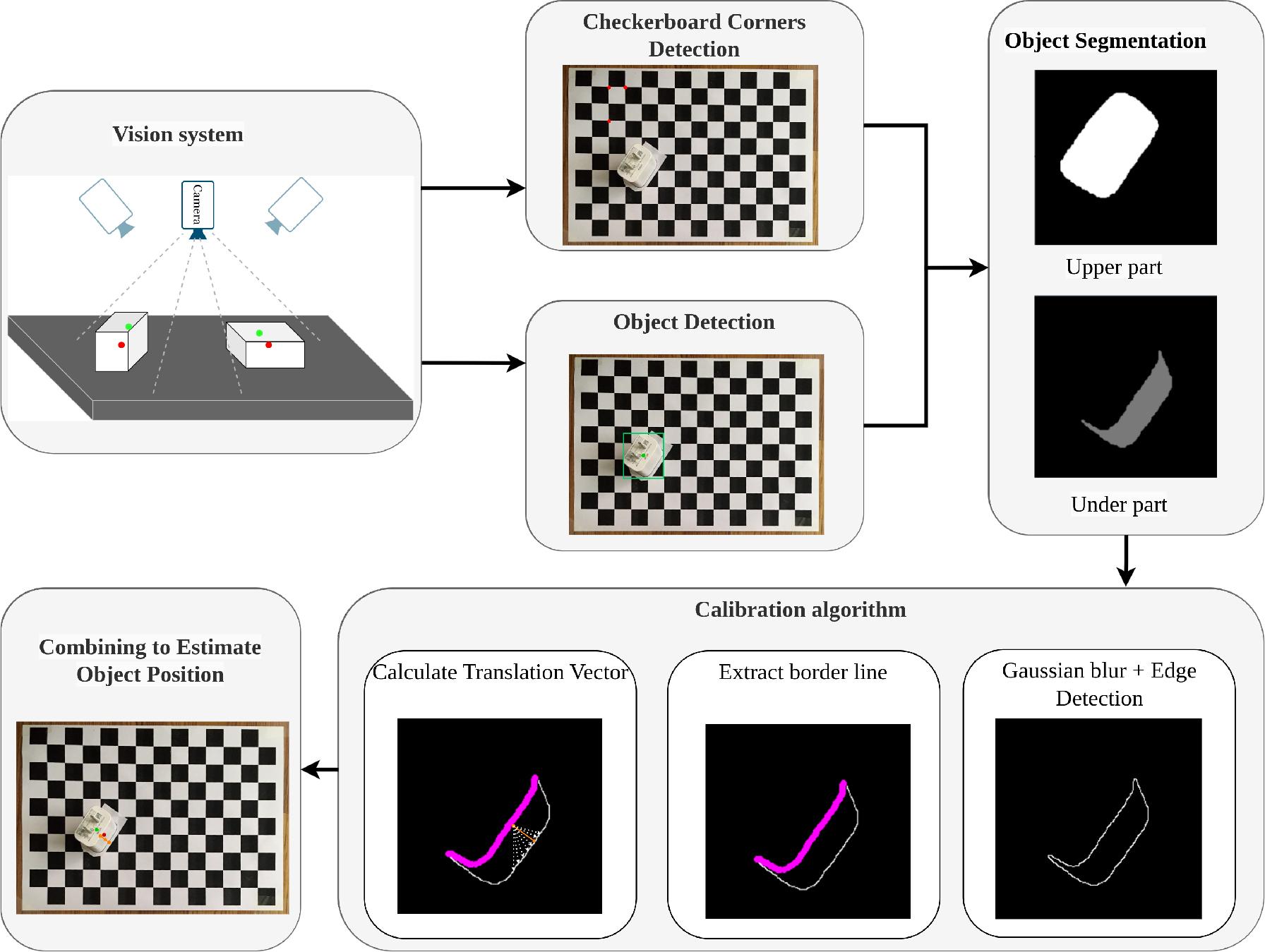
A block diagram of our proposed calibration method. The translation vector between the initialized estimate center point (green point), and the calibration center point (red point) is calculated based on deep learning, and our novel calibration method
Firstly, the checkerboard pattern demonstrates robustness against scenes that are out of focus [31]. Secondly, the features extracted from the checkerboard offer a straightforward definition of the original coordinate, contrasting with asymmetric circle patterns, where features are more suitable for motion determination. The checkerboard pattern plays a pivotal role in precisely determining the object’s position in the calibration process. As the monocular cameras sweep the calibration pattern, known as Or corner, we leverage the You Only Look Once (YOLO) model [32], a state-of-the-art object detection model, to identify objects within the camera’s field of view. Once the fixed original coordinate is defined, sub-pixel localization accuracy is crucial for extracting the image centers of the calibration targets to optimize sensor calibration. This process is detailed in Section 3.1. However, owing to the direction of light, the object’s position may drift away from the actual center. To address this, we introduce a novel calibration method comprising two parts. Initially, we segment the object into the upper plane (Su) and the lower plane (S1), as discussed in Section 3.2, utilizing the Bilateral filtering algorithm to eliminate noise. Subsequently, we determine the center of the upper plane (Pu) and employ an edge detection algorithm to extract the edge (E0) of the lower part. This edge (E0) is then divided into two main border lines: the upper line (Eu) and the lower line (E1). The translation vector (T) from (Eu) to (Et) is calculated, as detailed in Section 3.3. Finally, the estimated object position is computed by shifting the center of the upper part (Pu) following the translation vector (T) with a magnitude of 1/2.
In determining the precise position of the object, we initiate the process by establishing real-world coordinates through the capture of a checkerboard image, enabling the identification of its corners. Subsequently, for each object present in the image, we leverage an advanced object detection method to discern their respective image coordinates. In the context of detecting checkerboard corners, we establish the correlation between the image coordinates and their corresponding real-world coordinates. Notably, the relationship between distances in images and their counterparts in the real world is not always linear due to distortion. Figure 4 delineates the sequential steps employed to ascertain the initial object position:
Detect Checkerboard Edges and Corners: Utilizing the Hough transformation, we identify checkerboard edges and the coordinates of their intersections, namely, checkerboard corners, as depicted in Figure 4a.
Select Fixed Real-World Coordinate: Choose a fixed real-world coordinate in pixel image space, denoted as Or = [x0 y0]T.
Estimate Object Center Position: Employing object detection, estimate the center position in pixel image space, represented as P = [x y]T.
Calculate Object Position in Real-World Coordinates: Compute the object’s position in real-world coordinates using the formula Pr = (P – Or)r signifies the average ratio between the length in pixels and the length in the real world of each cell in the checkerboard pattern.
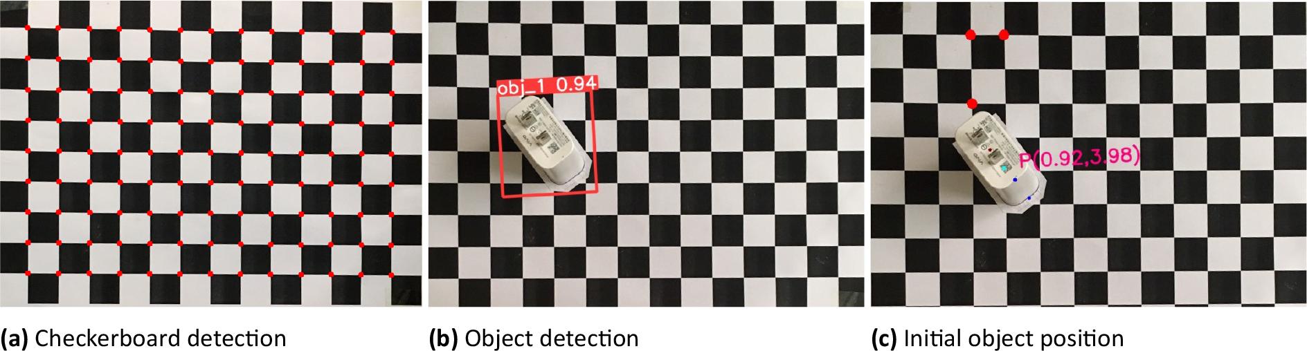
The progress of the calculation of the object position in the real-world coordinate
While utilizing the checkerboard calibration method to estimate the location of objects proves to be straightforward and readily applicable in industrial settings, its efficacy diminishes significantly when dealing with 3D-shaped objects. In instances involving such objects, the bounding box generated through deep learning methods may not align accurately with the true object location.
Specifically, the coordinates of the bounding box’s center are unlikely to correspond to the actual center of the object within the resultant image. It’s crucial to note that the bounding box’s center can accurately represent the object’s center only if the object is precisely positioned at the center of the camera’s projection onto the floor. To address this limitation, we employ a convolutional neural network (CNN)based object segmentation approach to divide objects, detected in Section 3.1, into two distinct planes. This segmentation involves using the upper plane Su to establish the initial center of the object, followed by noise reduction and edge extraction from the lower plane.
The initial step involves applying a Bilateral filtering operation, which can be expressed mathematically as:
where:
- -
I'(p) is the filtered intensity at pixel p.
- -
Wp is the normalization term.
- -
I(q) is the intensity at pixel q.
- -
Gσs is the spatial Gaussian kernel with standard deviation σs.
- -
Gσr is the range Gaussian kernel with standard deviation σr.
- -
Ω is the spatial neighborhood of the pixel p.
Here, k is the size of the kernel, and σ is the standard deviation of the Gaussian distribution.
After that, the edge detector includes gradient computation, non-maximum suppression, and edge tracking by hysteresis. The magnitude of the gradient (G) and the gradient direction (θ) are calculated as follows:
Then we divide the edge into two main border lines: the upper line (Eu) and the lower line (El). The upper line is the contact line between the two planes Su and Sl, and the lower line is the boundary of the lower plane Sl. Figure 5 illustrates the progress of object segmentation and edge extraction.
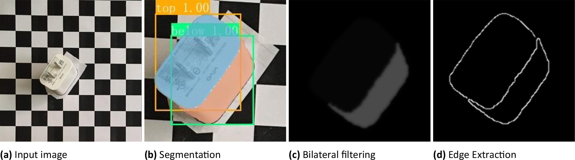
The progress of object segmentation and edge extraction
We introduce a calibration technique designed for object position calibration. Upon completion of the object segmentation and edge extraction processes, we obtain crucial components: the initial position of the object (center of the upper plane Su), the upper line Eu, and the lower line El. The translation vector Vul is then calculated using Algorithm 1 to predict the final position of the object by shifting the initial point according to Vul. In this process, each point on the upper line Eu calculates its distance to the lower line Sl, determining the smallest vector length. The visualization results are depicted in Figure 6a. Subsequently, the translation vector Vul is defined as the vector with the maximum length within the set of distance vectors for each point, as illustrated in Figure 6b.
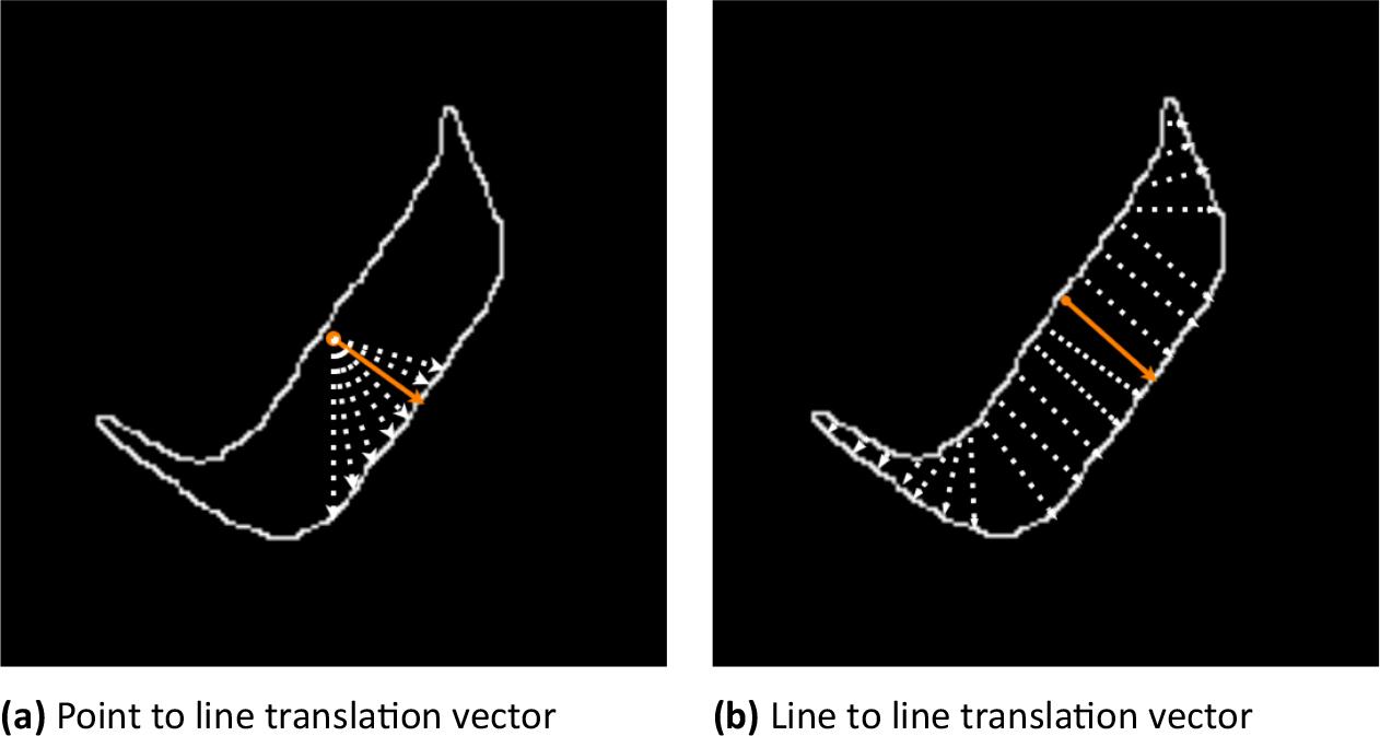
Illustration of the estimated translation vector
Input: 𝒫u = Eu1,Eu2,…,EuN
𝒫l = El1,El2,…,ElM
N is the number of points in line Eu
M is the number of points in line El
Output: Translation vector:
Index point in line Eu: indu
Index point in line El: indl
begin:
i ← 0 ;
j ← 0 ;
indu, indl ← 0 ;
𝒟EuEl ← 0 ; ▷ The magnitude of the translation vector
while i < (N – 1) do
𝒟iEl ← +∞; ▷ The distance from a point to a line
while j < (M – 1) do
Calculate the distance between two points (Pui = (xui, yui)) and (Plj = (xlj, ylj)) based on (4):
if 𝒟iEl ≥ D then
DiEl ← D;
end
j+ = 1;
end
if DEuEl ≤ DiEl then
DEuEl ← DiEl;
indu ← i;
indl ← j;
end
i+ = 1;
end
return
end
This calibration technique facilitates accurate object positioning by accounting for the spatial relationships between the upper and lower components. However, the efficacy of Algorithm 1 can be compromised by suboptimal segmentations. To mitigate this issue, we introduce Algorithm 2 as a solution. In essence, if the vector Vul derived from Algorithm 1 is accurate, then upon projecting the upper line Eu along the translation vector, the distance between the resultant line Ŝu and the lower line Sl should be approximately, or equal, to 0.
Leveraging this concept, we construct the set of neighboring vectors 𝕍 by maintaining the initial point of the vector Vul unchanged and selecting k neighboring points for the terminal point. Subsequently, we project the upper line following each translation vector in 𝕍 and choose the vector that results in the smallest distance.
This novel algorithm serves to enhance the robustness of the calibration process against suboptimal segmentations, ensuring more reliable results.
To evaluate the proposed method for estimating the location of objects, we conducted experiments using a vision system with a camera positioned above, parallel to the floor, and at a distance of 40cm. The real-world coordinates were defined using a checkerboard pattern, where each square was measured 3 × 3cm2. Further details about the experimental setup, including hardware specifications, are provided in Table 1. In our experiments, we used a specific type of object to evaluate the performance of our localization algorithm. The object selected for this study is a standard electrical charger, commonly found in households and industrial settings. This object was chosen due to its well-defined shape and easily recognizable features, which facilitate accurate detection and segmentation. The dimensions of this object are 4.5cm × 3.0cm × 3.5cm. The dimensions, shape, and sharpness of the localized object significantly impact the performance of the localization algorithm. The object’s well-defined edges and distinct features enable the deep learning models to accurately detect and segment it from the background. The size of the object ensures that it is neither too small to be overlooked by the detection model.
Experiment setup details
| Parameter Spec | Spec |
|---|---|
| Process | Intel Xeon Processor with two cores @ 2.3 GHz |
| GPU | NVIDIA Tesla T4 |
| RAM | 13 GB |
| OS | Ubuntu 20.04 LTS |
The rectangular shape with flat surfaces and sharp edges facilitates precise boundary detection during the segmentation process. The clear and distinct contours of the object enhance the segmentation accuracy, leading to better calibration results.
The evaluation metrics employed for a comprehensive assessment are Intersection over Union (IOU) for object segmentation, Mean Average Precision (mAP) for object detection, and the Euclidean metric for geometric accuracy.
We utilize a set of robust metrics to assess the performance of our proposed object localization method thoroughly. The Intersection over Union (IOU) metric, pivotal in the object segmentation phase, is defined as the ratio of the area of overlap (Aol) between predicted (Apred) and ground truth (Agt) bounding boxes to the area of union (Aun):
The mean average precision (mAP) is utilized for the object detection phase, calculated by integrating the precision (P) over the recall (R) and the number of classes at various IOU thresholds:
Input: 𝒫u = Eu1,Eu2,…,EuN
𝒫l = El1,El2,…,ElM
N is the number of points in line Eu
M is the number of points in line El
Output: Translation vector:
begin:
▷ Choose k neighboring points of 𝒫lindl
i ▷ –k/2 ;
𝕍 ← {}; ▷ Set of translation vectors
while i < k/2 do
j ← indl + i;
𝕍. pushback
end
𝒟min ← +∞;
for j = 0; j < size(𝕍); j + + do
▷ Calculate the distance between
𝒟 ← 0;
n ← 0;
m ← 0;
while n < (N – 1) do
while m < (M – 1) do
Calculate the distance d between two points
(Plm = (xlm, ylm)) based on (4);
D ← D + d;
m+ = 1;
end
n+ = 1;
end
if 𝒟min ≥ 𝒟 then
𝒟min ← 𝒟;
end
end
return
end
The Euclidean metric assesses geometric accuracy by calculating the Euclidean distance dEuclidean between the predicted ((Xpred,ypred)) and true ((xtr, ytr)) object coordinates:
We acquired three distinct datasets, each corresponding to a specific phase of our paper. In the object detection phase, we amassed a collection of 400 images captured from various object locations. To ensure a comprehensive evaluation, we partitioned this dataset into three subsets: a training set comprising 60% of the data randomly selected, a validation set with 30%, and a test set with the remaining 10%. Subsequently, in the object detection phase, we gathered 5000 images from diverse object locations. To maintain a robust evaluation approach, we split this dataset into a training set (70% of the data randomly selected), a validation set (20%), and a test set (10%). Lastly, for the object localization phases, we gathered 60 images, distributed into 10 folds, each containing 6 images.
Table 2 presents the results of various detection models evaluated in terms of mean average precision – mAP, model size – MS (MB), precision – Pr, and recall – Rc. The Yolov3 [33] model achieves a mAP of 90.0% with a model size of 8.7 MB, accompanied by precision and recall scores of 85.9% and 84.6%, respectively. In contrast, the Fast R-CNN [34] model demonstrates superior performance with a mAP of 97.0% despite a larger model size of 12.9 MB, achieving precision and recall scores of 93.4% and 42.1%, respectively. The MobileNet [35] model offers a mAP of 94.8% with a relatively compact model size of 4.6 MB, achieving precision and recall scores of 93.8% and 93.4%, respectively. The Yolov4 [36] and RTMDet [37] models exhibit competitive mAP scores of 96.8% and 96.9%, respectively, with larger model sizes of 60.0 MB and 52.3 MB. The Yolov7 [38] and Yolov8 [39] models can achieve superior accuracy with a mAP of 97.1% and 97.8%, respectively, with a precision of 95.7% and 95.5%, and a recall of 93.1% and 94.4%, respectively. Our proposed model outperforms the others with an mAP of 98.7%, precision of 98.6%, and recall of 97.0%.
Performance comparison of various object detection models
| Algorithm | mAP | Pr | Rc | MS |
|---|---|---|---|---|
| RTMDet [37] | 96.9% | 94.5% | 93.1% | 52.3 |
| MobileNet [35] | 94.8% | 93.8% | 93.4% | 4.6 |
| Fast R-CNN [34] | 97.0% | 93.4% | 94.1% | 12.9 |
| Yolov3 [33] | 96.3% | 95.8% | 95.7% | 8.7 |
| Yolov4 [36] | 96.8% | 96.6% | 95.4% | 60.0 |
| Yolov7 [38] | 97.1% | 95.7% | 93.1% | 37.2 |
| Yolov8 [39] | 97.8% | 95.5% | 94.4% | 11.1 |
| Our | 98.7% | 98.6% | 97.0% | 7.0 |
Additionally, our model exhibits a relatively compact size of 7.0 MB compared to other models, indicating its efficiency in terms of memory usage. These results underscore the effectiveness and efficiency of our proposed object detection model for accurately detecting objects in various scenarios, making it well-suited for practical deployment in real-world applications.
A comparative analysis of various object segmentation models is presented in 4. Among the models evaluated, Yolov5 [40] emerges as a strong contender, showcasing a notable mAP@0.5 score of 98.7%, a precision rate of 97.1%, and a recall rate of 96.2%. These metrics indicate its robust ability to accurately identify objects within images while maintaining a relatively compact model size of 7.4 MB, making it an efficient choice for resource-constrained environments. In addition, Yolov7 [38] and Yolov8 [39] demonstrate a commendable performance with high mAP scores of 99.0% and 99.2%, respectively, along with impressive precision and recall values. However, what sets our proposed model apart is its exceptional performance across all metrics. With an outstanding mAP@0.5 score of 99.8%, precision rate of 99.1%, and recall rate of 97.9%, our model surpasses all others in terms of segmentation accuracy while maintaining a moderate model size of 28.9 MB. These results underscore the efficacy of our segmentation model in accurately delineating objects within images.
Figure 7 visually illustrates the experimental results of our proposed method, including object detection, object segmentation, and object calibration. These visualizations provide a comprehensive insight into the efficacy and accuracy of each phase of our methodology. Object detection showcases the ability of our model to accurately identify and localize objects within the scene, laying the foundation for subsequent processing steps. Object segmentation highlights the precision with which our algorithm delineates the boundaries of detected objects, ensuring accurate localization and analysis. Finally, object calibration visually demonstrates the refinement and optimization of object positions based on real-world coordinates, validating the effectiveness of our calibration approach in enhancing spatial accuracy.
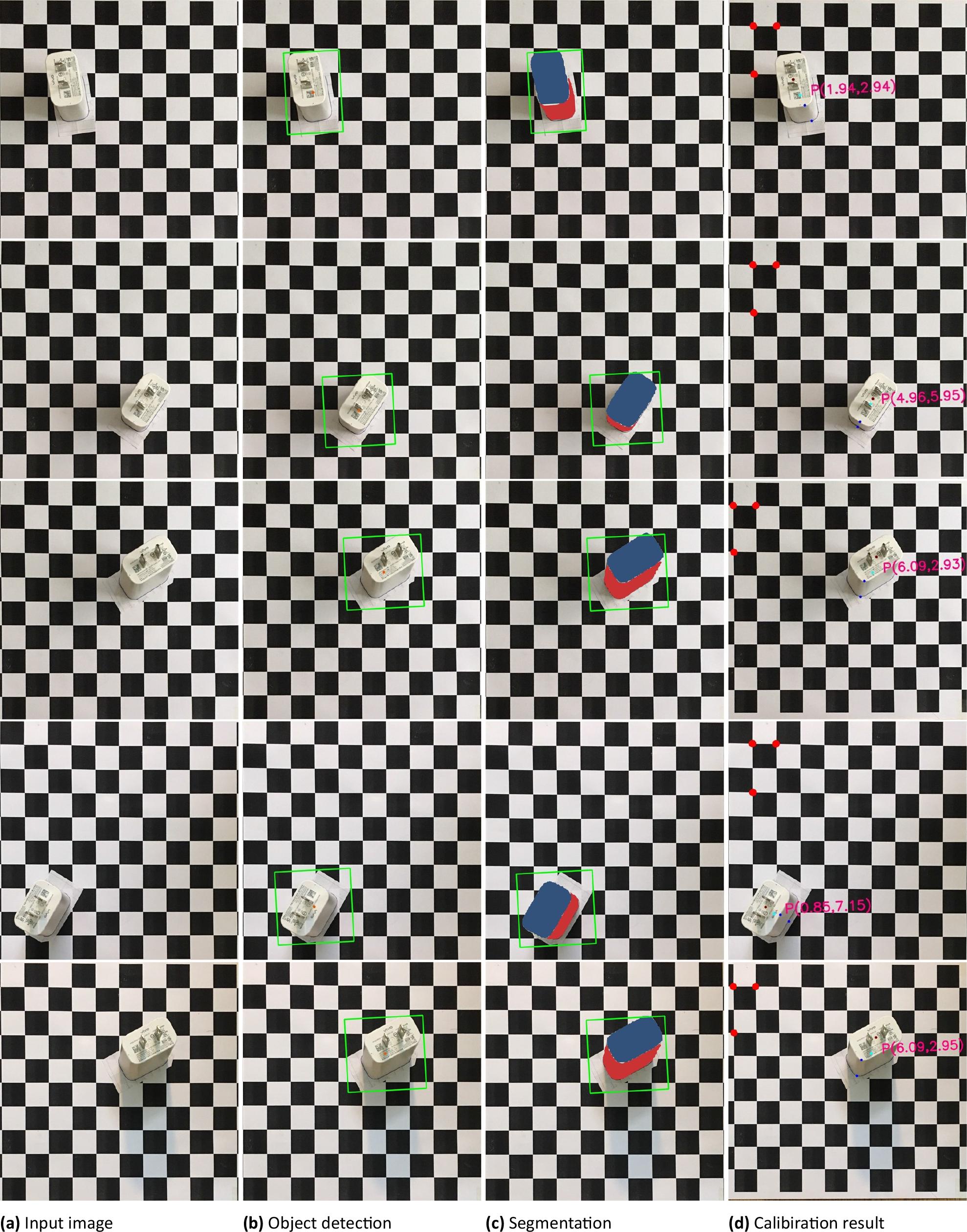
Visualized examples of experimental results: figure (b): the orange point is the Yolo center, figure (d): dark red is the upper part center. The vector created by the blue points is a translation vector; the light blue point is the correction center
The experimental results in Table 3 offer quantitative insights into the performance comparison between our proposed method, the traditional approach, and the Regression-based method [30], our previous method [30] (Regression-based method). Across multiple folds and samples, our method consistently demonstrates superior performance in terms of position error metrics.
Experimental results evaluate the position error of our algorithm (mm)
| Fold | Sample | Traditional Method | Regression Method [30] | Proposed Method | |||||||||
|---|---|---|---|---|---|---|---|---|---|---|---|---|---|
| Δx | Δy | Err | Δx | Δy | Err | Δx | Δy | Err | Δx | Δy | Err | ||
| 1 | 1 | 9.69 | 5.51 | 11.15 | 1.34 | 1.32 | 1.88 | 0.38 | 1.14 | 1.20 | 0.95 | 0.76 | 1.22 |
| 2 | 8.36 | 8.74 | 12.09 | 1.92 | 2.50 | 3.15 | 3.04 | 1.33 | 3.32 | 1.71 | 1.33 | 2.17 | |
| 3 | 5.13 | 8.93 | 10.30 | 1.23 | 1.52 | 1.96 | 1.14 | 0.95 | 1.48 | 1.14 | 0.95 | 1.48 | |
| 4 | 10.07 | 8.36 | 13.09 | 1.79 | 1.97 | 2.66 | 1.14 | 1.33 | 1.75 | 1.52 | 1.33 | 2.02 | |
| 5 | 8.55 | 10.26 | 13.36 | 0.75 | 1.12 | 1.35 | 0.76 | 0.19 | 0.78 | 0.38 | 0.57 | 0.69 | |
| 6 | 9.31 | 9.31 | 13.17 | 0.96 | 1.41 | 1.71 | 0.19 | 1.52 | 1.53 | 0.57 | 0.76 | 0.95 | |
| 2 | 1 | 4.18 | 5.89 | 7.22 | 1.45 | 3.07 | 3.40 | 1.33 | 2.09 | 2.48 | 0.95 | 1.14 | 1.48 |
| 2 | 10.07 | 13.11 | 16.53 | 3.12 | 3.41 | 4.62 | 2.47 | 1.71 | 3.00 | 2.47 | 1.33 | 2.81 | |
| 3 | 3.42 | 7.03 | 7.82 | 1.21 | 2.78 | 3.03 | 1.52 | 1.90 | 2.43 | 0.76 | 0.57 | 0.95 | |
| 4 | 10.07 | 8.74 | 13.33 | 2.13 | 1.51 | 2.61 | 0.95 | 0.19 | 0.97 | 1.90 | 0.95 | 2.12 | |
| 5 | 11.02 | 12.16 | 16.41 | 2.94 | 2.67 | 3.97 | 2.28 | 1.71 | 2.85 | 2.47 | 0.57 | 2.53 | |
| 6 | 8.93 | 11.02 | 14.18 | 0.43 | 1.34 | 1.41 | 1.33 | 0.38 | 1.38 | 0.19 | 0.19 | 0.27 | |
| 3 | 1 | 9.12 | 7.60 | 11.87 | 1.39 | 1.42 | 1.99 | 0.95 | 0.19 | 0.97 | 1.14 | 0.38 | 1.20 |
| 2 | 4.18 | 13.87 | 14.49 | 2.54 | 3.36 | 4.21 | 3.23 | 0.19 | 3.24 | 2.28 | 0.57 | 2.35 | |
| 3 | 9.88 | 4.18 | 10.73 | 0.76 | 1.12 | 1.35 | 0.57 | 0.76 | 0.95 | 0.57 | 0.76 | 0.95 | |
| 4 | 7.60 | 8.93 | 11.73 | 1.89 | 2.17 | 2.88 | 1.71 | 0.95 | 1.96 | 1.71 | 0.95 | 1.96 | |
| 5 | 10.45 | 4.94 | 11.56 | 0.88 | 2.34 | 2.50 | 1.71 | 1.52 | 2.29 | 0.57 | 0.76 | 0.95 | |
| 6 | 6.08 | 7.60 | 9.73 | 0.36 | 0.57 | 0.67 | 0.19 | 0.57 | 0.60 | 0.19 | 0.57 | 0.60 | |
| 4 | 1 | 13.87 | 10.26 | 17.25 | 1.37 | 2.84 | 3.15 | 0.76 | 2.47 | 2.58 | 0.95 | 2.09 | 2.30 |
| 2 | 11.97 | 7.98 | 14.39 | 2.84 | 1.45 | 3.19 | 2.28 | 1.33 | 2.64 | 2.28 | 1.33 | 2.64 | |
| 3 | 5.32 | 4.56 | 7.01 | 0.35 | 0.81 | 0.88 | 0.19 | 0.38 | 0.42 | 0.19 | 0.57 | 0.60 | |
| 4 | 5.51 | 16.34 | 17.24 | 0.32 | 1.32 | 1.36 | 0.76 | 1.14 | 1.37 | 0.19 | 1.71 | 1.72 | |
| 5 | 10.26 | 8.36 | 13.23 | 0.92 | 0.92 | 1.30 | 2.28 | 0.76 | 2.40 | 0.57 | 1.14 | 1.27 | |
| 6 | 6.27 | 11.40 | 13.01 | 1.47 | 1.63 | 2.19 | 1.90 | 2.85 | 3.43 | 1.33 | 1.33 | 1.88 | |
| Average | 8.30 | 8.96 | 12.54 | 1.43 | 1.86 | 2.34 | 1.38 | 1.15 | 1.92 | 1.12 | 0.94 | 1.55 | |
Performance comparison of various object segmentation models
| Algorithm | mAP | Pr | Rc | MS (MB) |
|---|---|---|---|---|
| Yolov5 [40] | 98.7% | 97.1% | 96.2% | 7.4 |
| RCNN [41] | 97.8% | 98.1% | 96.4% | 16.8 |
| Yolov7 [38] | 99.0% | 99.0% | 97.8% | 37.9 |
| Yolov8 [39] | 99.2% | 98.7% | 97.4% | 11.8 |
| Our | 99.8% | 99.1% | 97.9% | 28.9 |
For instance, in Fold 1, Sample 1, the traditional method yields position errors of Δx = 9.69 mm and Δy = 5.51 mm, while our proposed method achieves significantly lower errors of Δx = 0.38 mm and Δy = 1.14 mm before correction, and Δx = 0.95 mm and Δy = 0.76 mm after correction.
The average position errors across all folds and samples further highlight the effectiveness of our proposed method. On average, our method achieves position errors of Δx = 1.12 mm and Δy = 0.94 mm after correction, compared to Δx = 8.30 mm and Δy = 8.96 mm for the traditional method, which reduces the position error by 87.64%. Similarly, the regressionbased method yields average errors of Δx = 1.43 mm and Δy = 1.86 mm, indicating a noticeable improvement over the traditional approach but still inferior to our proposed method.
These quantitative results underscore the significant reduction in position errors achieved by our proposed method compared to both traditional and regression-based approaches. The superior accuracy and precision offered by our method are particularly advantageous in applications where precise object localization is paramount, such as robotic manipulation, augmented reality, and autonomous navigation systems.
The processing time for each phase of our proposed method is summarized in Table 5. In the object detection phase, our algorithm takes approximately 15 ± 2 milliseconds to detect objects within the camera’s field of view. Subsequently, during the object segmentation phase, which involves segmenting the detected objects into upper and lower planes, the algorithm also requires around 40±5 milliseconds. Finally, in the object calibration phase, where the precise position of the objects is determined based on the segmented data, the processing time remains consistent at approximately 300 ± 10 milliseconds. This efficient processing time across all phases underscores the real-time applicability and practical feasibility of our proposed method for object localization in industrial vision systems.
Processing time of our proposed method (milliseconds)
| Phase | Processing Time |
|---|---|
| Object Detection | 15 ± 2 |
| Object Segmentation | 40 ± 5 |
| Object Calibration | 300 ± 10 |
In conclusion, we have presented M-Calib, a comprehensive methodology for precise object localization and calibration leveraging advanced computer vision techniques for industrial robot vision systems.
Through the integration of advanced computer vision techniques, including object detection, segmentation, and calibration, our proposed approach offers a robust and accurate solution for determining the real-world positions of objects. Experimental results demonstrate the effectiveness of our method in significantly reducing 87.65% position errors compared to traditional approaches, thereby enhancing spatial accuracy in industrial environments. Furthermore, the computational efficiency of our method, as evidenced by minimal processing times, underscores its practical viability for real-world deployment. Overall, our proposed methodology holds promise for a wide range of industrial applications where precise object localization is essential, offering a reliable solution to optimize operational efficiency and enhancing productivity. In the future, our aim is to explore machine learning techniques for automatic calibration parameter adjustment and extend our methodology to support realtime dynamic object localization.