
The growing demand for efficient and reliable electric drives has intensified research on sensorless control techniques, which estimate rotor position from current and voltage measurements instead of physical sensors. Common approaches include the model reference adaptive system (MRAS), the extended Kalman filter (EKF), electromotive force (EMF) estimation and high-frequency signal injection (HFI). Each technique offers specific advantages depending on the motor topology and speed range (Belghazali et al., 2025; Janiszewski, 2023; Ran et al., 2025; Rodriguez-Montero et al., 2021; Sandre-Hernandez et al., 2019; Zuo et al., 2023). The HFI method is particularly effective at zero and low-to-medium speeds, as it injects a high-frequency signal into the stator windings and utilises the rotor’s magnetic anisotropy to estimate position through current variations along the direct (d) and quadrature (q) axes. Field-oriented control (FOC) is typically employed as the main framework, enabling independent control of flux and torque components while enhancing HFI performance without direct position feedback (Ferdiansyah and Hanamoto, 2024; Lu et al., 2022; Matsuo and Lipo, 1993; Prystupa et al., 2023; Wang et al., 2022, 2023). In several studies, interior-rotor permanent magnet-assisted synchronous reluctance motors (PMaSynRMs) have employed real-time automatic tuning of the band-pass filter (BPF) and continuous monitoring-based control of the estimated angle error to improve the accuracy of rotor position estimation (Akgul et al., 2022). Similarly, for synchronous reluctance motors (SynRMs), various approaches adapt the injection amplitude according to instantaneous load, stabilising current components and improving robustness (Chen et al., 2024b; Li et al., 2020). Furthermore, hybrid sensorless control structures combining adaptive HFI at low speeds with EMF-based models at higher speeds have enabled full-speed-range operation (Lu et al., 2018; Ohnuma et al., 2014). Nevertheless, such adaptive HFI strategies have not yet been investigated for outer-rotor permanent magnet-assisted synchronous reluctance motors (OR-PMaSynRMs).
PMaSynRM motors have attracted increasing interest due to their high efficiency, low rotor losses and suitability for sensorless control. By reducing magnet volume through reluctance torque production, they achieve cost and thermal advantages while maintaining adequate torque at low current levels, thereby improving overall efficiency (Jani and Jamnani, 2023; Zhao et al., 2025). The outer-rotor topology considered in this study increases torque with the rotor diameter, enhancing torque density per unit volume. However, the extended magnetic flux path in this configuration reduces the saliency ratio compared with interior-rotor machines, making current responses less distinctive for rotor position estimation in HFI-based methods and limiting their applicability (Bozkurt et al., 2021). To enable effective HFI implementation in OR-PMaSynRMs, adaptive mechanisms for frequency, amplitude and filtering are required. The amplitude adaptation approach dynamically adjusts the injected signal according to operating conditions. This method stabilises the high-frequency current response and improves position estimation accuracy, provided that the signal amplitude remains below the voltage saturation limit (Alberti et al., 2017; Kang and Lorenz, 2018; Setty et al., 2013; Tongxing et al., 2019). Adaptive frequency control, on the other hand, adjusts the injection frequency to prevent interference with the fundamental component and noise coupling. Several studies have proposed dynamic tuning strategies to optimise estimation accuracy (Lee et al., 2024; Pan et al., 2016). The adaptive adjustment of demodulation filter cut-off frequencies according to signal variations is also essential. Matching the filter cut-off with the injection frequency enables precise current separation, while proportional tuning minimises coupling with fundamental components and improves stability (Chen et al., 2024b; Sun et al., 2022). Since adaptive HFI performance depends on machine parameters, the strategy must be individually optimised for each motor. Although previously applied to other configurations, it has not yet been implemented in OR-PMaSynRMs. In this study, the injection parameters were experimentally identified for the target motor and drive system. Additionally, a voltage limiting mechanism was developed to prevent saturation by continuously monitoring the total voltage vector and dynamically rescaling its magnitude when the threshold is reached, thus maintaining signal integrity and enhancing position estimation accuracy.
The contributions of this study to the literature can be summarised as follows:
The control parameters required for efficient and stable operation of the OR-PMaSynRM, previously unexamined using the HFI method, were experimentally identified and compared with similar approaches applied to other motor types.
Under dynamic operating conditions, the injection frequency, amplitude and demodulation filter cut-off were adaptively tuned, and an HFI-based sensorless control algorithm was developed specifically for the OR-PMaSynRM.
A novel active voltage limiting method was proposed to enhance position estimation accuracy. The developed scheme was experimentally implemented and its effectiveness was verified.
Reluctance-based motors are promising candidates for sensorless control due to their simple structure, low losses and high efficiency (Mishra, 2023). Compared with conventional SynRM, PMaSynRMs achieve higher torque density and improved efficiency by utilising rotor-embedded magnets that enhance magnetic flux and enable the generation of both reluctance and magnet torque (Diao et al., 2023; Hsieh et al., 2022; Murataliyev et al., 2022).
For effective control design, it is essential to have a clear understanding of the motor’s magnetic and electrical behaviour. The motor’s behaviour can be characterised in the dq reference frame through voltage, flux and torque equations, and its equivalent circuit is shown in Figure 1.
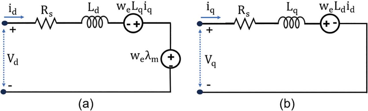
Equivalent electrical circuit representation of the OR-PMaSynRM in the dq reference frame: (a) d-axis model, (b) q-axis model. OR-PMaSynRM, outer-rotor permanent magnet-assisted synchronous reluctance motor.
In the equivalent circuit, Rs denotes the stator resistance, while Ld and Lq represent the dq-axis inductances, respectively. Based on this model, the electrical equations for the OR-PMaSynRM can be derived as follows:
In Eqs (1) and (2), Vd and Vq denote the stator voltages, id and iq are the current components, λd and λq represent the flux linkages in the dq-axes and ωe is the electrical angular speed of the rotor as follows:
In Eq. (4), λq represents the total flux linkage along the q-axis, expressed as a non-linear function of the stator current components id and iq. The term λq0 denotes the q-axis flux linkage component that arises solely from the reluctance effect, excluding the influence of the permanent magnet flux. λm corresponds to the permanent magnet flux aligned with the q-axis. Under weak saliency, the reduced difference between Ld and Lq limits the distinctness of current responses, making rotor position estimation more difficult (Wu et al., 2017) as follows:
In Eq. (5), the electromagnetic torque (T) comprises the reluctance torque, caused by the flux difference between the dq-axes, and the magnet torque, generated by the permanent magnets. Here, P denotes the number of poles, and λPM represents the magnet flux.
The structural comparison between the outer and inner rotor configurations is illustrated in Figure 2. Saliency refers to the difference in magnetic properties between the dq-axes of the motor and serves as an indicator of the magnetic anisotropy resulting from the rotor geometry. As the difference between the dq-axis inductances increases, the magnetic orientation disparity and the saliency level of the rotor become more pronounced.
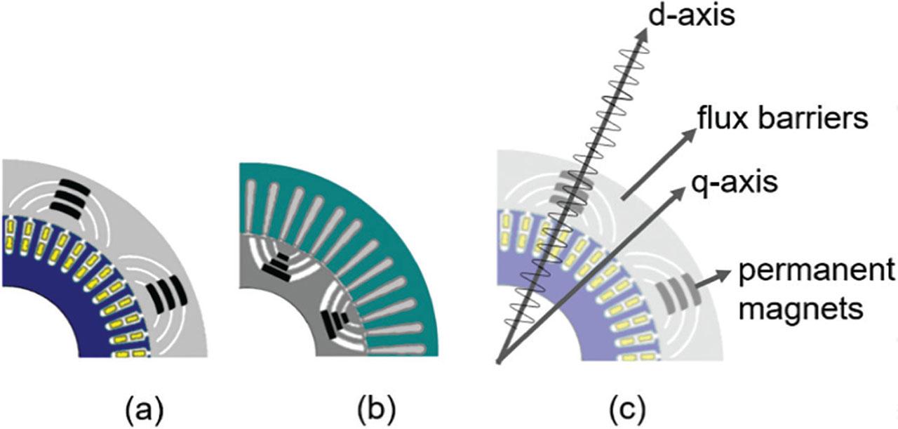
Cross-sectional views of PMaSynRM with (a) outer rotor and (b) inner rotor configurations. PMaSynRM, permanent magnet-assisted synchronous reluctance motors
Figure 3 shows the electromagnetic analysis of the OR-PMaSynRM. The motor’s saliency ratio (ξ = Lq/Ld) is approximately 2.58, indicating low magnetic saliency. The reduced inductance difference (Ld − Lq) caused by the outer rotor design limits conventional sensorless control performance, especially at low and zero speeds. Although HFI relies on magnetic anisotropy for position estimation, weak current responses in low-saliency motors reduce accuracy and increase control complexity, requiring adaptive control strategies.
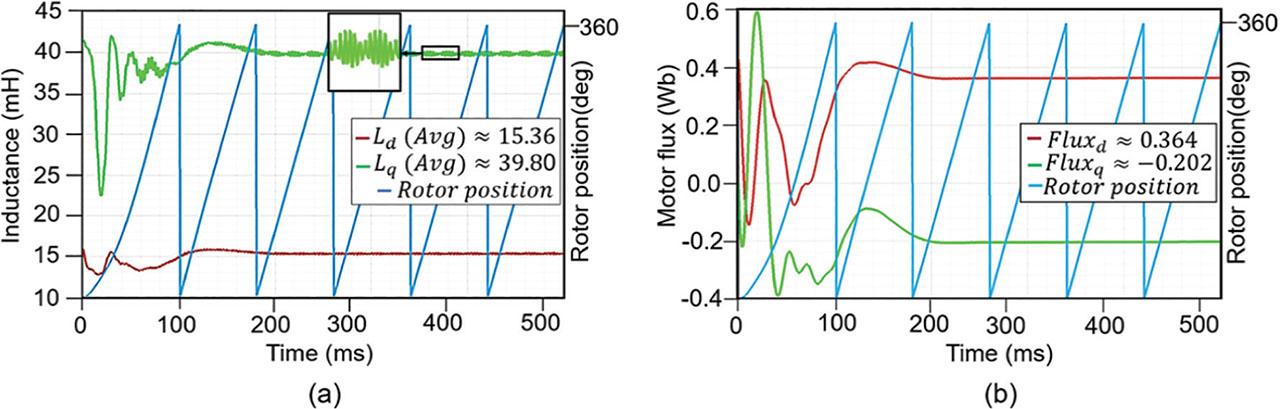
Electromagnetic characteristics of the OR-PMaSynRM: (a) Variation of the Ld and Lq inductances with respect to the rotor position and (b) magnetic flux linkage characteristics of the motor and the rotor position graph. OR-PMaSynRM, outer-rotor permanent magnet-assisted synchronous reluctance motor.
In HFI methods, the rotor position is estimated by applying a high-frequency voltage signal to the stator windings. The injected excitation interacts with the motor’s intrinsic magnetic anisotropy and produces high-frequency current components whose amplitude and phase characteristics carry information related to the rotor position. In the conventional rotating-frame HFI approach, the high-frequency excitation is applied in the dq reference frame, thereby stimulating both axes simultaneously, and can be expressed as follows:
In contrast, the pulsating HFI method adopted in this study injects the high-frequency voltage solely into the d-axis, while the q-axis component is kept at zero, and yields as follows:
This simplified d-axis injection is preferred because the d-axis aligns with the dominant saliency direction, resulting in a clearer and more distinguishable position dependent current response. Injecting a high-frequency signal into the q-axis, by contrast, would disrupt the torque producing current and increase torque ripple. Thus, d-axis pulsating excitation avoids such undesirable effects and offers clear advantages for OR-PMaSynRM machines, where saliency is naturally weaker. When the high-frequency voltage is applied to the d-axis, the measured currents include rotor position dependent high-frequency components (Jiang et al., 2024; Lu et al., 2021). In this context, the dq-axis high-frequency voltage components and the angular frequency of the injected signal are denoted by
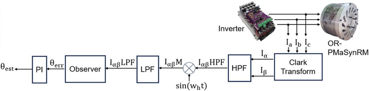
The phase currents (Ia, Ib, Ic) are processed through several stages, as shown in Figure 4. The measured currents are transformed into the stationary reference frame components (Iα, Iβ) using the Clarke transformation. High-pass filter (HPF) is then applied to extract the high-frequency components, yielding the filtered signals (IαβHPF). These signals are modulated with a sinusoidal reference to obtain the modulated currents (IαβM). Finally, a low-pass filter (LPF) isolates the position-dependent component (IαβLPF), which is used by the observer to estimate the rotor position (θest). Although this method is effective under certain conditions, its reliance on fixed signal parameters reduces stability under load variations and speed fluctuations. Therefore, adaptive HFI strategies based on frequency, amplitude and voltage adaptation have been developed to ensure reliable performance. The HPF removes the DC offset and low-frequency components of the measured current, allowing only the high-frequency components to pass through. The LPF, in turn, suppresses the high-frequency components and extracts the low-frequency signal containing rotor position information. This enhances the sensitivity of demodulation and maintains the stability of the estimated signal. Figures 5a and 5b show the discrete-time structures of the first-order digital HPF and LPF used in the demodulation stage.
Demodulation stages in HFI-based rotor position estimation. HFI, high-frequency signal injection; HPF, high-pass filter; LPF, low-pass filter.
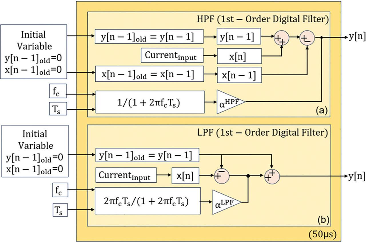
Implementation structures of the first-order digital filters: (a) HPF used in the demodulation stage, (b) LPF used in the signal extraction stage. HPF, high-pass filter; LPF, low-pass filter.
In HFI-based sensorless control, reliable extraction of rotor position-dependent current components necessitates adaptive adjustment of the signal parameters. Without proper adaptation, frequency mismatches may occur, leading to degraded estimation accuracy and reduced control performance as follows:
Eq. (8) presents the mathematical expression of the applied high-frequency adaptation. In this equation,
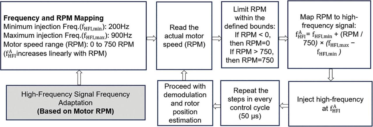
Flowchart of the adaptive frequency injection algorithm.
Although adaptive frequency enhances the separation of rotor-position-dependent components, it is not sufficient on its own. As the injection frequency varies, the cut-off frequencies of the HPF and LPF must also be adjusted accordingly. Otherwise, fixed filters cause spectral overlap, allowing unwanted components or attenuating relevant signals. Adaptive filtering, tuned according to motor speed and injection frequency, improves noise suppression at low speeds while preserving signal integrity at high speeds, thereby enhancing the reliability of rotor position estimation.
Accurate extraction of current components containing rotor position information requires dynamic adjustment of the signal amplitude. A fixed amplitude, regardless of load or speed variations, may either weaken the injected signal or introduce noise under excessive levels. This condition reduces the accuracy of position estimation and negatively affects overall system stability. Adaptive amplitude adjustment responds to these varying conditions, improving the signal-to-noise ratio and enhancing estimation accuracy as follows:
Eq. (9) presents the mathematical expression of the applied high-frequency signal amplitude adaptation. In this equation,
Figure 7 shows the process flow of high-frequency signal amplitude adaptation based on motor load. The motor current is measured, the load ratio is calculated and the injection amplitude is adjusted in real time according to this ratio.

Flowchart of the adaptive injected signal amplitude control.
The key contribution of the proposed voltage-limiting structure lies in its ability to dynamically account for the additional voltage component arising from the adaptive nature of the HFI. Conventional voltage-limiting methods in the literature define the voltage boundary solely as a function of the DC-bus voltage and the fundamental FOC control action, implicitly assuming a constant-amplitude injection signal. In contrast, the HF amplitude in this study is adaptively varied in real time to enhance rotor-position estimation accuracy. As a result, classical limiting strategies become inadequate when the HF component increases the total voltage magnitude. The proposed method updates the voltage limit according to both the fundamental control terms and the instantaneous HF amplitude, ensuring that the Vout vector remains within the inverter boundaries and that the adaptive HFI mechanism operates stably. In this respect, the method provides a novel and necessary improvement over fixed-amplitude assumptions commonly adopted in prior work.
In the HFI strategy, maintaining the integrity of the injected signal is essential for accurate rotor position estimation. However, the inverter’s DC bus limits the maximum output voltage, thereby constraining the total stator voltage vector (Vout). In adaptive HFI control, Vout consists of the d-axis component (Vd), the q-axis component (Vq) and the high-frequency signal (VHFI) superimposed on the d-axis. Under high-load conditions, the combined magnitude of these components may exceed the DC bus limit, affecting system stability. To prevent this, a real-time adaptive voltage limiting strategy has been developed, ensuring that the VHFI signal remains within safe voltage margins. This approach preserves both control stability and position estimation accuracy.
Figure 8 shows the effect of the proposed voltage-limiting strategy on Vout in the αβ (alpha–beta) reference frame. In Figure 8a, VHFI is superimposed on the Vd component, and together with Vq, it forms the Vout vector. This vector exceeds the reference voltage boundary (Vref (max)) defined by the inverter’s DC-bus voltage (Vin). Exceeding this boundary reduces control accuracy and may lead to errors in rotor position estimation. Figure 8b illustrates the condition after applying the proposed voltage-limiting strategy. Once the overshoot is detected, the Vout vector is dynamically rescaled while preserving its phase angle. Consequently, a new vector, Vout (lim), is obtained within the permissible voltage region. The limited voltage components, Vd (lim) and Vq (lim), are recalculated to maintain the integrity of the superimposed VHFI signal as follows:

(a) Total stator voltage vector exceeding the voltage limit and (b) limited stator voltage vector.
Eqs (11)–(13) define the mathematical relationships used to calculate the total stator voltage magnitude, the inverter’s maximum reference voltage and the phase angle of the voltage vector. Eq. (11) expresses the mathematical formulation of Vout, where Vd total corresponds to the sum of Vd and VHFI, while Vq total corresponds to Vq. Eqs (12) and (13), respectively, provide the mathematical expressions for the maximum permissible reference voltage Vref (max) and the phase angle θv, derived from the dq-axis voltage components.
Figure 9a presents a detailed vector representation of the proposed voltage limiting strategy, illustrating the error magnitude and corresponding correction mechanism when Vout exceeds Vref (max). The Vd and Vq components combine with the VHFI signal applied along the d-axis to form the total voltage vector Vout. When this vector surpasses Vref (max), the exceeding portion is identified as the error vector (VErr), defined by its magnitude and direction. This vector is decomposed into dq components, VErr·cos(θv) and VErr·sin(θv), which represent the excess voltage contributions along the respective dq-axes. These components are subtracted from the original voltage references to ensure that the resultant vector remains within the inverter’s permissible range. Accordingly, the limited d-axis voltage Vd (lim) is obtained by subtracting VErr·cos(θv) from (Vd + VHFI), while the limited q-axis voltage Vq (lim) is derived by subtracting VErr·sin(θv) from Vq. As a result, Vout (lim) is rescaled within the inverter voltage boundary while preserving its phase angle.
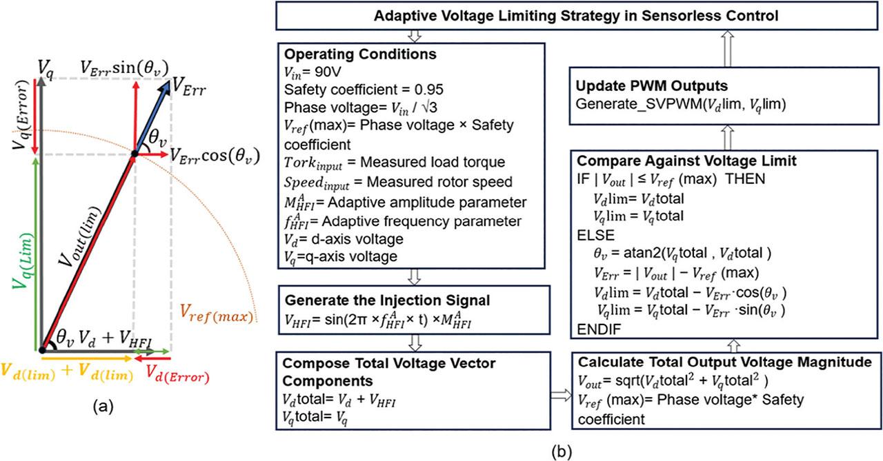
(a) Vector representation of the proposed limiting strategy based on error vector decomposition and (b) flowchart of the adaptive voltage limiting strategy. SVPWM, Space Vector Pulse Width Modulation.
Figure 10a presents all parameters of the proposed adaptive HFI method in a block module form. As this module is part of the integrated control structure shown in Figure 12, its internal configuration is detailed here. Figure 10b illustrates the computational flow diagram of the proposed adaptive voltage limiting algorithm. This diagram summarises the real-time mathematical processing steps performed to ensure that the total output voltage vector remains within the inverter’s permissible range.
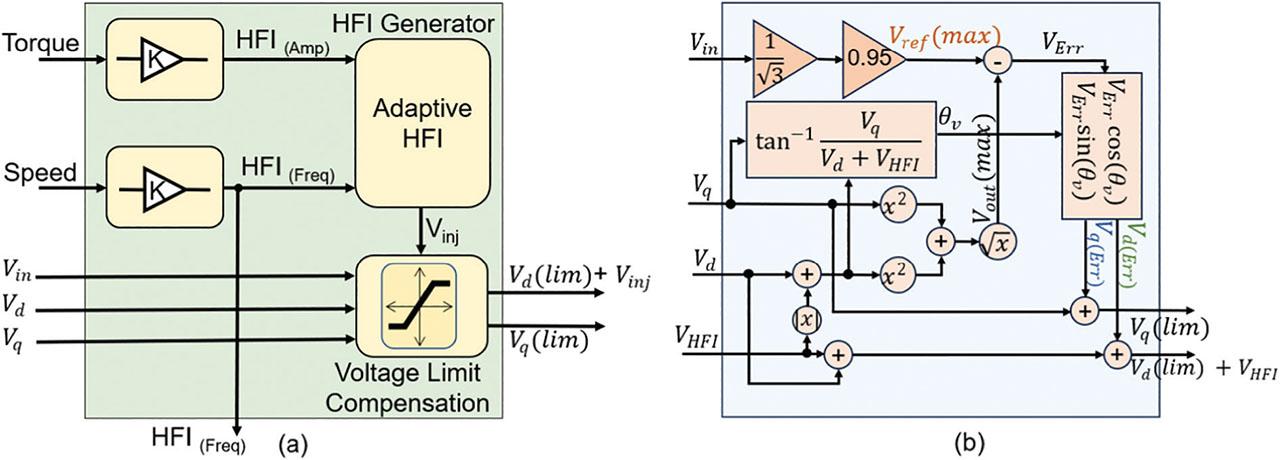
(a) Adaptive HFI signal generation and voltage limiting block and (b) mathematical flow diagram. HFI, high-frequency signal injection.
Figure 11 illustrates the dynamic behaviour of the output voltage components before and after activation of the voltage limiting strategy. During the initial interval (t < t0), where t denotes the system time and t0 represents the instant at which the strategy is enabled, the output voltage Vout periodically exceeds the inverter’s permissible limit, generating the error voltage VErr. This overflow distorts the trajectory of the voltage vector. As shown, the error components Vd (Err) and Vq (Err) represent the voltage overflow along the dq-axes and occur as a result of saturation. When the voltage limiting algorithm is activated at t = t0, the voltage vector is dynamically reshaped and confined within the safe operating region defined by Vref (max). The dq-axis voltage components are updated in real time, resulting in the limited vectors Vd (lim) and Vq (lim). This process preserves the VHFI signal applied on the d-axis, maintaining signal integrity and compatibility with the inverter’s voltage capacity. Consequently, estimation stability is improved without transient distortion. The proposed voltage limiting structure enables the motor drive to operate within the inverter’s voltage boundaries while preserving VHFI signal integrity, thereby enhancing the accuracy and reliability of sensorless rotor position estimation. The signal shown in Figure 11 was captured in real time from the computer interface connected to the operating motor drive.
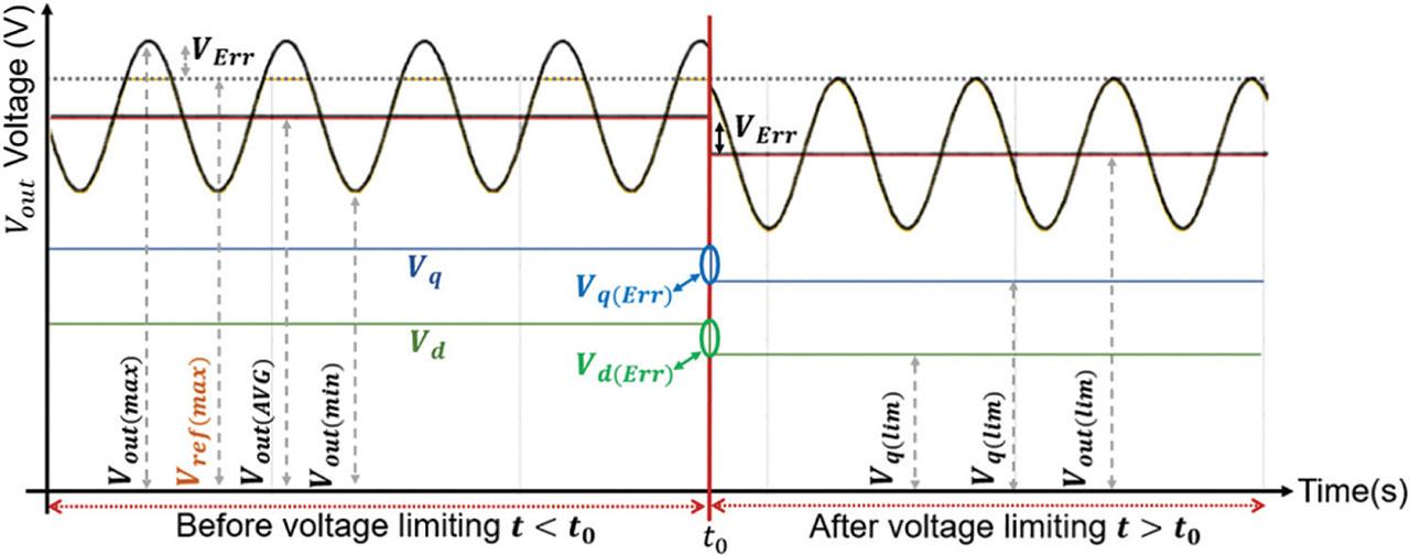
Comparison of the VHFI signal integrity before and after the voltage limiting.
Figure 12 illustrates the overall signal flow within the control structure. The difference between the reference and actual phase currents is processed by the PI controllers to generate the Vd and Vq components. These voltages, together with the reference speed, torque and Vref (max), are supplied to the block that performs adaptive HFI control and voltage limiting. Within this block, the adaptive HFI mechanism and the injected VHFI signal generate the limited voltage components Vd (lim) and Vq (lim).These components are converted into Va, Vb and Vc through inverse Park and Clarke transformations and are then applied to the Space Vector Pulse Width Modulation (SVPWM) module to produce the inverter switching signals. The adaptive HFI block dynamically adjusts the cut-off frequencies of the demodulation filters according to the injection frequency, thereby maintaining accurate signal extraction under varying operating conditions.
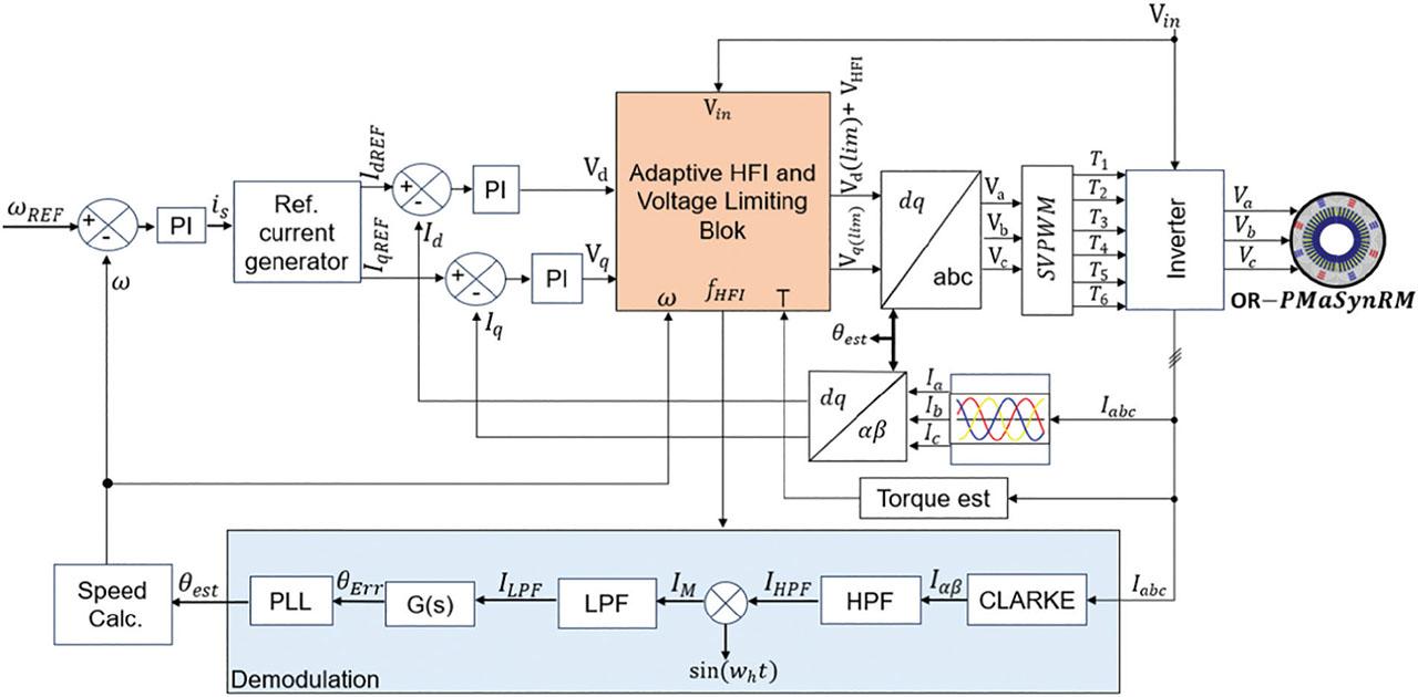
Block diagram of the FOC-based adaptive HFI sensorless control system. FOC, field-oriented control; HFI, high-frequency signal injection; HPF, high-pass filter; LPF, low-pass filter.
Figure 13 present the experimental set-up and schematic representation of the developed sensorless OR-PMaSynRM drive system. The DC power supply provides the input voltage to the inverter, while the motor drive circuit performs the control and switching operations. The isolated ST-Link programmer ensures electrical isolation between the computer and the system, allowing controller programming. The digital oscilloscope monitors system signals in real time, and the current probe measures the phase currents. The computer functions as both the control interface and the data acquisition unit. The loading unit enables testing of the motor under various load conditions.
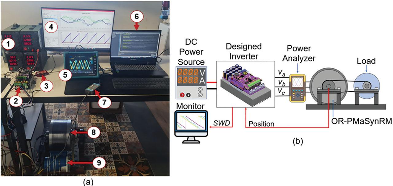
(a) The established OR-PmaSynRM sensorless drive system: (1) DC power source, (2) motor drive circuit, (3) isolated ST-Link, (4) monitor, (5) digital oscilloscope, (6) PC, (7) current probe, (8) OR-PmaSynRM, (9) current brake and (b) the OR-PmaSynRM drive test unit. OR-PMaSynRM, outer-rotor permanent magnet-assisted synchronous reluctance motor.
During the experimental tests, the parameters of the hardware and software components forming the system are important. In this study, the data related to the hardware are summarised in Table 1, while the data related to the software are presented in Table 2. The limits of the adaptation parameters are listed in Table 3, and the technical parameters of the motor are provided in Table 4.
Experimental hardware specifications.
| Parameter | Value |
|---|---|
| Microcontroller | STM32F407VG (168 MHz, ARM Cortex-M4F [32-bit]) |
| DC bus voltage (Vin) | 90 VDC |
| Current sensor type | GHS 20-SME |
| Current sensor output sensitivity | 40 mV/A (typical) |
| Current sensing resolution | 12-bit ADC |
| Position sensor (for validation only) | MA702, 14-bit magnetic encoder |
| Cooling method | Aluminium heatsink and fan |
Experimental software specifications.
| Parameter | Value |
|---|---|
| Control method | FOC, HFI |
| HFI injection axis | d-axis only |
| Filter type (demodulation) | HPF and LPF (first-order digital) |
| Angle estimation method | PLL-based estimator with PI compensation |
| RMS angle error evaluation | RMSE |
| PWM switching frequency | 15 kHz |
| Proportional and integral gain values for the d-axis current controller
|
|
| Proportional and integral gain values for the q-axis current controller
|
|
FOC, field-oriented control; HFI, high-frequency signal injection; HPF, high-pass filter; LPF, low-pass filter.
Boundaries of adaptive control parameters.
| Control parameter | Adaptation variable | Operating range | Adaptive range |
|---|---|---|---|
| Adaptive injection frequency
| Motor speed (RPM) | 0–750 RPM | 200–900 Hz |
| Adaptive injection amplitude
| Load ratio (%) | 30%–60%–90% | 8–20 V |
| Adaptive filter cut-off frequency |
| – | 200–900 Hz |
| Reference voltage limit
|
| – | 45–49 V |
Specifications of the OR-PmaSynRM.
| Parameter | Value | Unit |
|---|---|---|
| Phase voltage | 90 | VRMS |
| Rated current | 5.741 | ARMS |
| Reactive power | 313 | VAR |
| Output power | 1500 | W |
| Input power | 1639 | VA |
| Efficiency | 91.51 | % |
| Rated speed | 750 | RPM |
| Frequency | 50 | Hz |
| Load torque | 19.1 | Nm |
OR-PMaSynRM, outer-rotor permanent magnet-assisted synchronous reluctance motor.
With its high processing capability and integrated peripherals, the STM32F407 microcontroller forms the core of the control architecture, providing a suitable structure for motor control applications. To reduce interference between the power and control stages, all digital signals are isolated through opto-isolators and isolated drivers. This hardware configuration provides a robust and noise-resilient platform for validating the proposed sensorless control under dynamic load conditions.
Based on the system parameters, several findings have been obtained from the experimental tests conducted to evaluate the performance of the adaptive HFI strategy. In this context, the responses observed during the frequency adaptation process reveal the system’s dynamic behaviour and the accuracy of rotor position estimation. The experimental results related to frequency adaptation are presented in Figure 14.
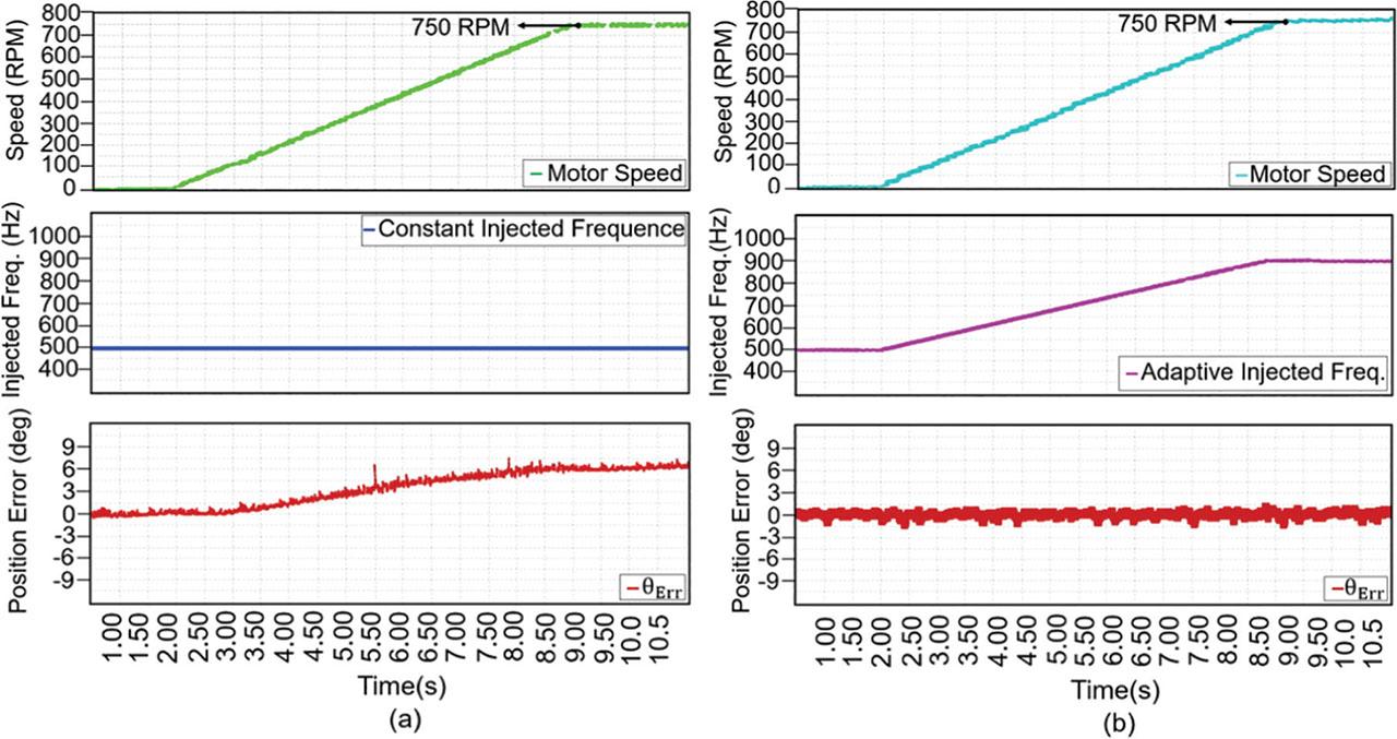
(a) Effect of a constant injection frequency on rotor position estimation error during motor speed increase and (b) impact of the adaptive injection signal frequency on rotor position estimation error during motor speed variations.
Figure 14a illustrates the condition in which the injected signal frequency was kept constant while the motor speed was gradually increased from 0 RPM to 750 RPM, with no adaptive mechanism applied. As the speed increased, the stator current spectrum expanded, overlapping with both the HFI frequency band and the motor’s inherent frequency components. Figure 14b, on the other hand, shows the adaptive adjustment of the injection frequency according to the motor speed. As the speed increased within the 0–750 RPM range, the injection frequency was updated based on experimentally determined threshold values. This approach preserved the integrity of rotor position-dependent information and improved demodulation accuracy. Following the frequency-adaptation stage, the motor speed was increased beyond its rated value to enable the transition into the flux-weakening region. This operating region is particularly important, as the reduction in effective magnetic flux at high speeds represents one of the most challenging conditions for maintaining the accuracy of rotor-position estimation methods. Consequently, the proposed approach was evaluated under reduced-flux conditions to assess its estimation performance.
In the flux-weakening region, the OR-PmaSynRM continues to operate stably, while the electrical angle and torque characteristics exhibit the expected behaviour associated with the reduction in effective magnetic flux. The electrical angle between the rotor flux vector and the stator current vector is referred to as the torque angle, and the quantity shown as “Angle Degree” in Figure 15 corresponds to this torque angle. When the torque angle is increased, the motor enters the flux-weakening region, and a reduction in the available torque occurs due to the applied voltage and current limitations. The experimental results presented in Figure 15 demonstrate that rotor-position estimation maintains its integrity throughout this operating range.
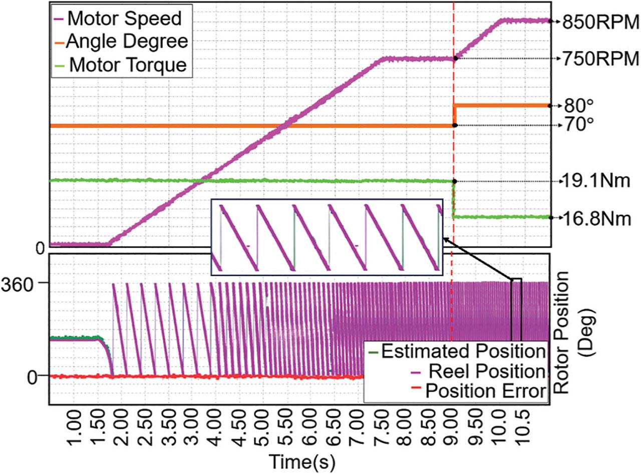
Flux weakening behaviour and rotor position estimation performance of the OR-PmaSynRM. OR-PMaSynRM, outer-rotor permanent magnet-assisted synchronous reluctance motor.
Figure 16a shows a condition in which the motor was operated at different load levels (30%, 60%, and 90%) while the amplitude of the injected signal was kept constant. As the load increased, the fundamental components of the phase current became dominant, weakening the effect of the fixed-amplitude high-frequency signal and causing a noticeable rise in position error. This indicates that the constant-amplitude strategy cannot maintain stability under varying load conditions. Figure 16b presents the same test performed with an adaptive amplitude adjustment according to the motor torque. As the load increased, the injection signal amplitude was proportionally adjusted, preserving the saliency-related current components and improving demodulation accuracy. Consequently, the position estimation error was significantly reduced compared with the fixed-amplitude condition.
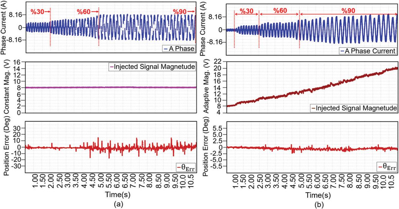
(a) Rotor position error resulting from a constant-amplitude injection signal under varying load conditions and (b) impact of the adaptive injection signal frequency on rotor position estimation error during motor speed variations.
Figure 17 shows the motor phase current waveforms measured under HFI. When the waveforms are examined, the injected high-frequency components are clearly visible in the current.
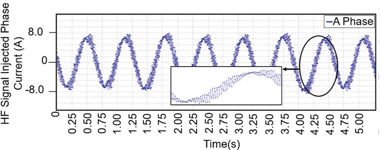
Motor phase current under high-frequency injection.
Figure 18 shows the Iα and Iβ current components obtained from the Clarke transformation of the phase currents. This operation represents the first step of the demodulation process. The resulting Iα and Iβ currents contain high-frequency components superimposed on the fundamental current waveform.

Iα and Iβ currents under high-frequency signal injection.
Figure 19 illustrates the waveforms of IαHPF and IβHPF, corresponding to the αβ current components after high-pass filtering. At this stage, HPF is applied to the Iα and Iβ signals to suppress the fundamental frequency components and extract the high-frequency content. As shown, the filtering process effectively eliminates the fundamental current component, thereby isolating the injected high-frequency signal for subsequent demodulation and position estimation.
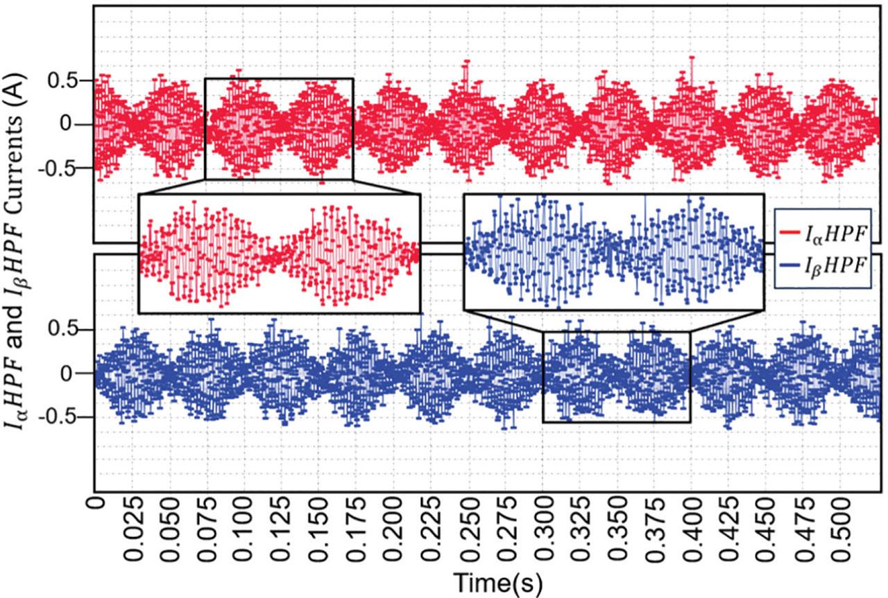
IαHPF and IβHPF signals obtained after the HPF stage. HPF, high-pass filter.
Figure 20 illustrates the modulated current signals, denoted as Iαmod and Iβmod, obtained through multiplication of the high-pass filtered currents with the injected high-frequency sine wave. During this modulation stage, the IαHPF and IβHPF components are synchronously multiplied by the same high-frequency carrier employed in the injection process. This operation enhances the saliency-related information and shifts the signal spectrum to a lower frequency band, thereby facilitating the subsequent demodulation stage.
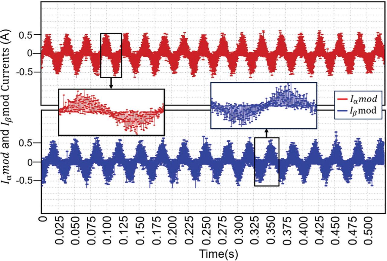
Outputs of Iαmod and Iβmod after sine-wave modulation.
Figure 21 presents the low-pass filtered current signals obtained following the modulation stage. In this stage, an LPF is applied to the Iαmod and Iβmod signals to extract the low-frequency envelope that carries the rotor position information. This filtering operation effectively suppresses the high-frequency carrier components, producing smooth and sinusoidal current waveforms, as illustrated in the figure. The resulting signals, IαLPF and IβLPF, are then used for precise rotor angle estimation.
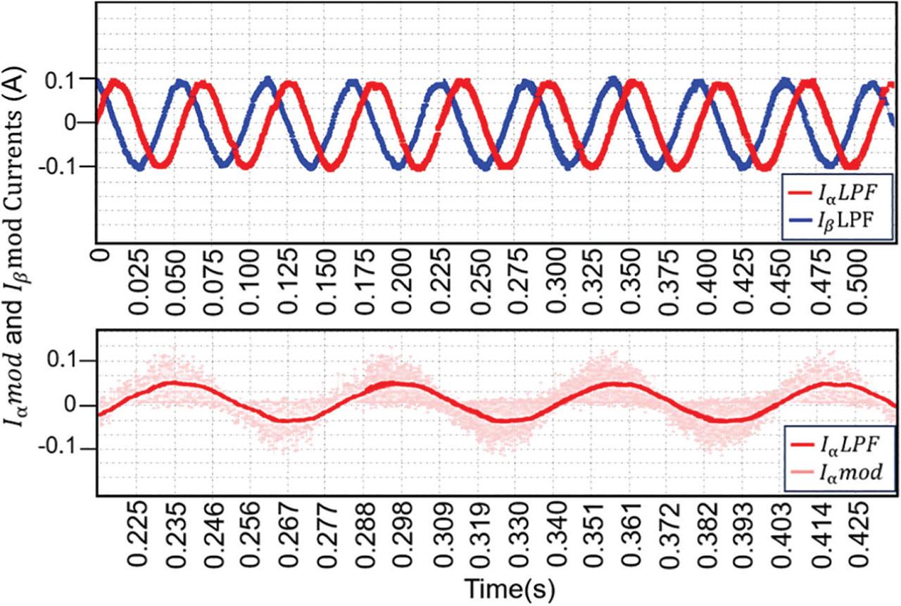
IαLPF and IβLPF current outputs obtained after low-pass filtering. LPF, low-pass filter.
To evaluate the effectiveness of the proposed sensorless method, the estimated rotor position was compared with the actual position measured by a magnetic encoder. As shown in Figure 22a, the estimated position closely follows the actual one throughout the entire operating period. The position error was calculated as the difference between the estimated and encoder-measured positions and expressed in electrical degrees. In Figure 22b, the motor was decelerated to a standstill while rotating at 250 RPM and then accelerated again in the opposite direction. Within this operating range, the actual and estimated rotor positions, together with the position error, are presented. The error remains within ±1.15° (electrical degrees), indicating that the proposed HFI method accurately tracks the rotor position with minimal deviation.
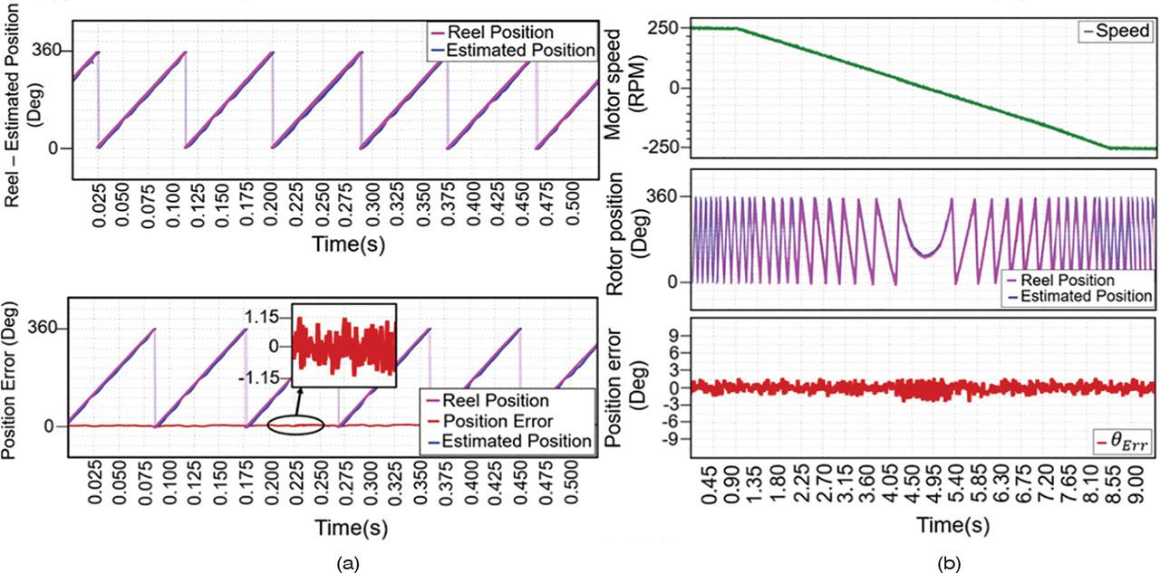
Rotor position estimation results: (a) Estimated rotor position compared with the real position and (b) rotor position estimation and corresponding error profiles under varying speed conditions.
Table 5 presents the RMS and maximum position estimation errors obtained under different operating conditions. The results show that the proposed adaptive HFI method provides stable and consistent estimation accuracy across the entire speed and load range. The RMS error remained approximately within ±1.15° electrical. Each experimental test was repeated three times under identical conditions to verify repeatability. The RMS position error values showed very small variation among trials, with the standard deviation ranging between ±0.02° and ±0.03° electrical. Considering the repeated short-term tests and the measurement noise level, the deviation was confirmed to remain below approximately ±0.03° under nominal operating conditions.
RMS position error under different operating conditions.
| Test condition | Motor speed (RPM) | Load torque (Nm) | RMS error (°electrical) | Standard deviation (°electrical) | Max error (°electrical) |
|---|---|---|---|---|---|
| Low speed, light load | 150 | ≈5.7 | 1.10 | ±0.02 | 1.23 |
| Medium speed, nominal load | 450 | ≈11.5 | 1.12 | ±0.02 | 1.28 |
| High speed, high load | 750 | ≈17.2 | 1.15 | ±0.03 | 1.35 |
During the rotor position estimation tests, additional experiments were conducted to further evaluate the performance of the proposed adaptive voltage limiting strategy. Figure 23 shows the system response with and without the voltage limiting enabled. The results demonstrate that rotor position estimation achieves higher accuracy, particularly during sudden load or speed variations. The signals were recorded in real time through the PC-based monitoring interface.

Impact of the proposed voltage limiting method on rotor position estimation.
Figure 23 (top plot) shows the Vout, obtained as the sum of Vd and Vinj components. When the motor operates under load without the proposed limiting strategy, Vout (max) exceeds the Vref (max) boundary, resulting in distortions in the IαHPF and IβHPF signals. These distortions, visible in the middle section of Figure 23, adversely affect the accuracy of rotor position estimation. Upon activation of the proposed limiting strategy, a noticeable improvement in the estimated position signal was achieved.
Table 6 presents a comparison of sensorless rotor position estimation methods applied to different motor types under FOC control. While most existing studies have focused on inner-rotor motors, the method proposed in this study has been specifically developed for the OR-PmaSynRM, which exhibits weaker magnetic saliency. As adaptive HFI studies for outer-rotor configurations remain limited in the literature, most compared methods are based on inner-rotor motor types.
Comparison of rotor position estimation errors reported in various studies.
| Study | Motor type | Control method | Estimation method | Average RMS error (electrical degrees) |
|---|---|---|---|---|
| Method in Chen et al. (2024a) | PMSM | FOC | Adaptive BPF + HFI | ≈1.2° |
| Method in Tap et al. (2023) | PmaSynRM | FOC | Adaptive HFI + modified PLL | ≈1°–1.5° |
| Method in Lu et al. (2018) | IPMSM | FOC | Adaptive frequency & amplitude HFI | <3° |
| Method in Chen and Liu (2012) | IPMSM | FOC | HFI | ≈±2° |
| Method in Tongxing et al. (2019) | PMSM | FOC | Frequency self-optimized HFI + PLL | ≈±14.4° |
| Method in Kumar et al. (2019) | IPMSM | FOC | HFI + Self-adaptive PLL + adaptive amplitude | ≈1.5° |
| My work | OR-PmaSynRM | FOC | HFI + adaptive frequency + adaptive amplitude + proposed voltage limiting | ±1.15° |
FOC, field-oriented control; HFI, high-frequency signal injection; OR-PMaSynRM, outer-rotor permanent magnet-assisted synchronous reluctance motor; PMaSynRM, permanent magnet-assisted synchronous reluctance motors.
In this study, an HFI-based sensorless rotor position estimation method was proposed and experimentally implemented for OR-PMaSynRM drives. The proposed method dynamically adjusts the injection frequency (200–900 Hz), signal amplitude (8–20 V) and the cut-off frequencies of the demodulation filters (200–900 Hz) in real time according to the operating conditions. In addition, an adaptive voltage-limiting strategy was developed to ensure that the total voltage vector remains within the inverter’s modulation capacity. Experimental results show that the proposed adaptive HFI algorithm significantly improves both position-estimation accuracy and control stability, particularly under low-speed and high-load conditions. The measured steady-state rotor position estimation error was obtained as an RMS value of approximately 1.15° electrical, with a standard deviation between ±0.02° and ±0.03° electrical. The maximum deviation remained below ±1.35° electrical throughout the entire speed range of 0–750 RPM. When the injection frequency or amplitude temporarily reached their adaptive limits, slight audible noise was observed in the motor, indicating that parameter adaptation is essential not only for maintaining estimation accuracy but also for preserving acoustic stability.