
1. Introduction
Titanium dental implant components combine threaded surfaces, shoulders, transitions, and mating features within a small three-dimensional volume. Their dimensional evaluation must retain information about the location and nature of geometric discrepancies. A global mean close to zero can conceal deviations of opposite signs in different regions, while a large maximum may represent a small isolated feature. Manufacturing feedback, therefore, requires both quantitative summaries and spatially resolved comparisons with the nominal geometry.
X-ray micro-computed tomography (micro-CT or μCT) provides volumetric data from which internal and external surfaces can be reconstructed. Kruth et al. [1] reviewed its use for dimensional quality control, including the measurement of features that are inaccessible to conventional coordinate measuring machines. Villarraga-Gómez et al. [2] compared X-ray CT and coordinate measuring machine (CMM) measurements of internal features and compliant structures. These applications demonstrate the value of CT for geometric inspection while emphasizing the need to assess its performance for the features and measurement conditions of interest.
Dimensional CT results depend on acquisition, reconstruction, surface determination, and subsequent geometric processing. Schlecht et al. [3] examined the influence of material thickness on CT-based dimensional measurements and found no significant effect under the conditions they studied. Carmignato et al. [4] used a traceable geometrical standard to assess errors of indication in X-ray microtomography. Dewulf et al. [5] developed a framework for evaluating uncertainty in dimensional CT measurements that, among other contributions, considers voxel-size calibration and edge determination. Thus, voxel size is an acquisition parameter, not by itself an estimate of measurement uncertainty. In the present application, the central challenge is to interpret μCT-to-CAD differences without attributing every observed discrepancy to the physical shape of the component.
The Guide to the Expression of Uncertainty in Measurement (GUM) [6] and the guidance on developing measurement models [7] provide a basis for relating a defined measurand to uncertain inputs. Statistical methods for processing and evaluating measurement results are discussed by Wimmer et al. [8]. In this application, a local surface-normal deviation, a radial difference, a fitted feature dimension, and a summary over a specified surface are distinct measurands. Their numerical values, and even the resulting ranking of components, may differ. The distinction between measurement precision and trueness is also relevant [9]: repeated numerical alignment of a single reconstructed surface characterizes only one part of the evaluation procedure.
The specific contribution of this study is an integrated, reproducible descriptive workflow: define the signed μCT-to-CAD nearest-surface deviation and its vertex weighting; compare complete D1–D3 exports by empirical distributions, common-scale histograms, diagnostic bands, and distributional distances; then localize the discrepancies within D1 and compare the interpretation with separately defined area-sampled and radial outputs. This combination identifies which findings depend on the chosen sampling and correspondence and where further feature-specific inspection is warranted. D1, D2, and D3 are separately measured components of the implant in Fig. 1, not independent production replicates.
The specific contribution of this study is an integrated and reproducible metrological and statistical workflow for μCT.
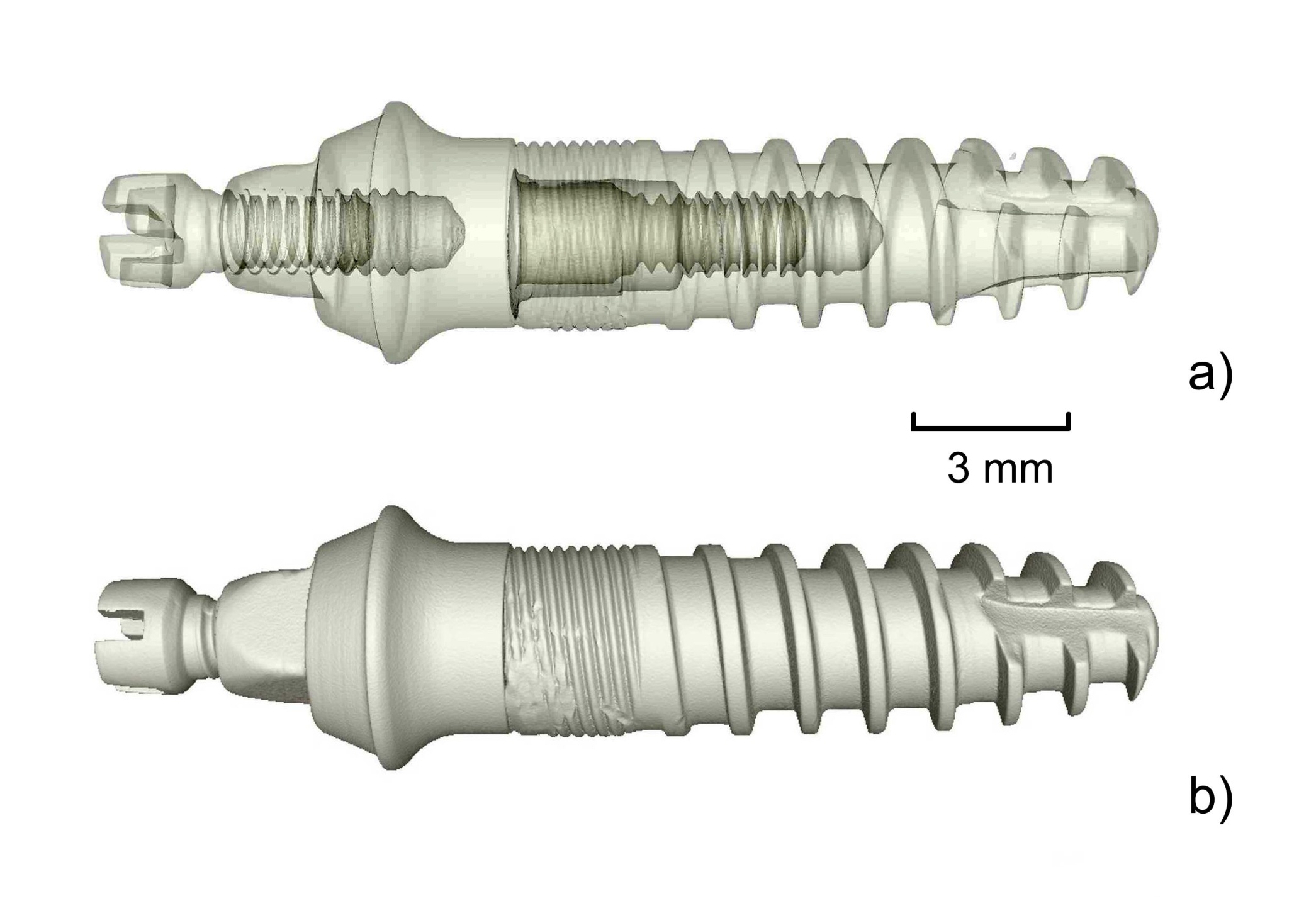
Fig. 1.
μCT-derived 3D model of the three-component titanium implant assembly: (a) semi-transparent rendering revealing the individual components; (b) opaque rendering. The scale bar indicates 3 mm.
2. Subject & Methods
A. Components and μCT measurement
The assembled implant and its three separately reconstructed components are shown in Figs. 1–4. Panels (a)–(c) of each component figure show the nominal CAD model, the μCT-derived STL surface, and a color-coded μCT-to-CAD deviation rendering, respectively. These renderings provide spatial context; the color scales are component-specific and do not permit direct numerical comparison between maps. The 3 mm scale bars apply to the component renderings. Because each component was aligned separately to its CAD reference, these comparisons do not preserve the relative positions of the components in the assembly.
Micro-CT measurements of the titanium implant components were performed using a Nanotom 180 X-ray microtomography system (GE Phoenix|X-ray, Germany). The scans were acquired with a voxel size of 13.75 μm and 1800 projections over a full 360° rotation. The X-ray tube was operated at 160 kV and 90 μA in measurement mode 0, without detector binning. A 0.2 mm copper filter was used to attenuate low-energy X-rays and limit beam-hardening effects. The detector exposure time was 750 ms per projection, and three-frame averaging was applied to reduce image noise. These acquisition settings do not, by themselves, establish dimensional accuracy or uncertainty [1, 5].
The projection data were reconstructed into three-dimensional volumes using datos|x 2.1 software (GE Sensing & Inspection Technologies GmbH, Germany) and the Feldkamp cone-beam reconstruction algorithm. The volumes were processed in VGSTUDIO MAX 2.0 (Volume Graphics GmbH, Germany). The same software isosurface threshold setting of 1/2 was applied in VGSTUDIO MAX to the reconstructed volumes of D1, D2, and D3 before STL export. This is a segmentation setting, not a dimensional calibration or an estimate of surface-location uncertainty; the corresponding absolute grey-level cut-off and the surface-determination implementation are not documented in the available exports. No systematic perturbation of the threshold was performed, so the sensitivity of the measured deviations to its choice remains unknown. Applying the same setting ensures a consistent processing choice but does not yield equal segmentation bias across components with different geometries [1, 5].
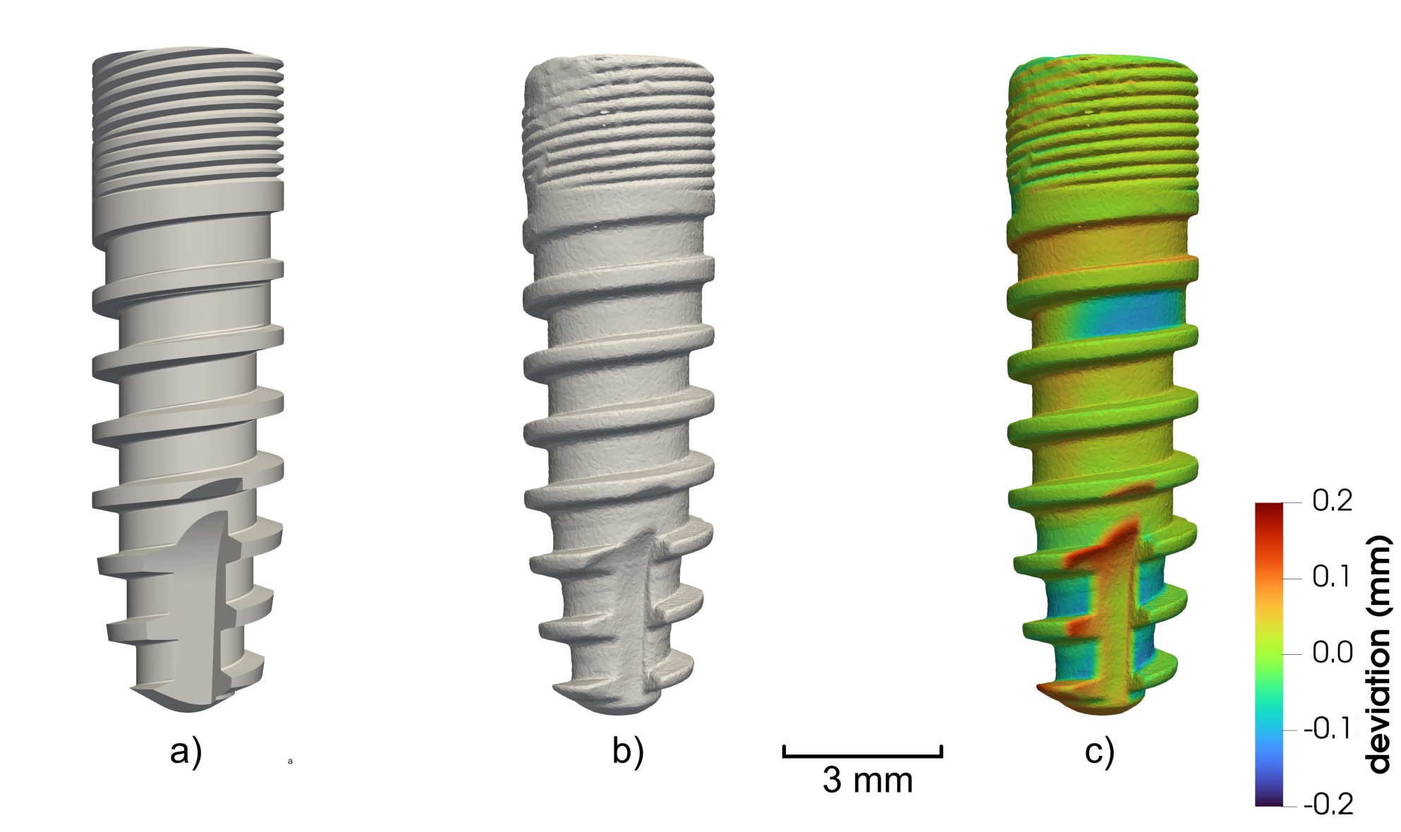
Fig. 2.
Component D1: (a) nominal CAD model; (b) μCT-derived STL surface; (c) supplied color-coded μCT-to-CAD deviation rendering. The scale bar indicates 3 mm and the displayed color represents ±0.2 mm deviation. Quantitative vertex summaries are calculated from the separate D1 export.
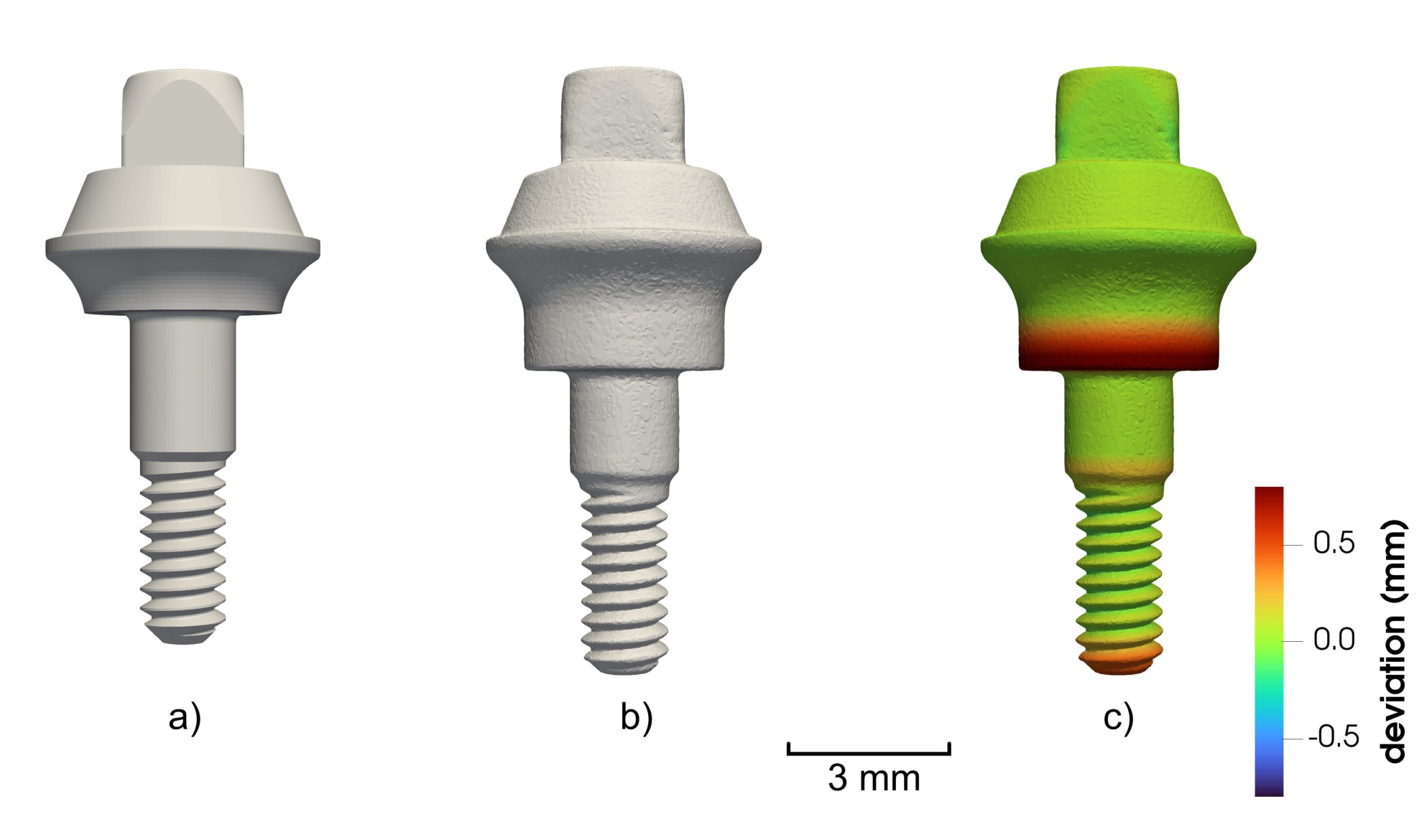
Fig. 3.
Component D2: (a) nominal CAD model; (b) μCT-derived STL surface; (c) supplied color-coded μCT-to-CAD deviation rendering. The scale bar indicates 3 mm, and the displayed color range represents ±0.7 mm deviation. The D1 and D2 colors represent different numeric scales.
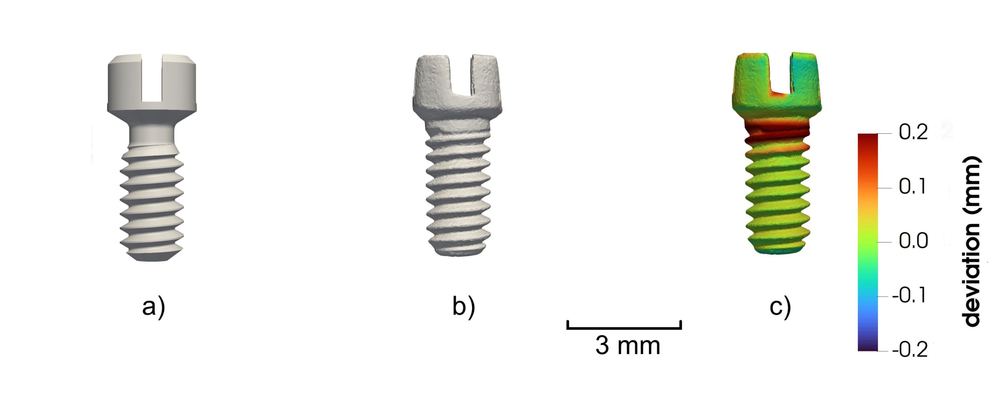
Fig. 4.
Component D3: (a) nominal CAD model; (b) μCT-derived STL surface; (c) supplied color-coded μCT-to-CAD deviation rendering. The scale bar indicates 3 mm, and the displayed color range represents ±0.2 mm deviation.
B. Registration and definition of vertex deviations
Each muCT-measured STL surface was registered independently to its corresponding manufacturer-controlled, component-specific CAD geometry. Its revision was fixed for the comparison and remains identifiable in the project records; the proprietary revision identifiers are not disclosed. The initial alignment used selected nominal reference features for each component, followed by a surface-based best-fit registration. The identities of those features, their construction datum, and the numerical initial and final transformations have not been released with the vertex exports. Consequently, a third party cannot reconstruct the registration uniquely from these tabular data.
The rigid transformation maps an original measured vertex xij of component j to
where Rj and tj denote the rotation matrix and translation vector, respectively.An automated coarse-to-fine registration procedure was developed to minimize operator-dependent errors and to accommodate large initial translations, substantial relative rotations, and geometrically repetitive features. First, the centroids of the μCT and CAD surfaces were aligned. To avoid bias caused by non-uniform STL mesh density, the centroids were estimated from STL surface points sampled randomly but uniformly with respect to triangle area rather than from a simple arithmetic mean of the STL mesh vertices, so that they are not biased by non-uniform mesh density.
Principal component analysis (PCA) was subsequently used to determine the principal axes of both surfaces. Because PCA does not uniquely determine the signs and, in geometrically ambiguous cases, the correspondence of the principal axes, 24 proper three-dimensional orientation hypotheses satisfying det(R) = 1 were considered.
To resolve ambiguous orientations, feature matching using Fast Point Feature Histograms (FPFH) combined with random sample consensus (RANSAC) was used to achieve a robust global alignment. This step was particularly important for component D2, exhibiting relatively large μCT-to-CAD geometric differences, and for component D3, for which a substantial initial relative rotation and symmetry had to be resolved.
The resulting transformation was refined using robust multi-scale point-to-plane iterative closest point (ICP) registration with Tukey loss function to reduce the influence of local geometric discrepancies and outliers. A numerical target distance of 0.005 mm was used as a stringent ICP convergence criterion. It was selected to keep numerical contributions associated with the iterative registration, including finite convergence and rounding effects, small relative to the spatial sampling scale of the μCT data. The criterion itself is not an estimate of registration or measurement uncertainty.
For each measured vertex of the registered μCT surface, the software determines the closest point cij on the corresponding CAD reference surface SCAD,j,
The corresponding signed nearest-surface deviation (signed nearest-surface Euclidean distance) is defined as
The sign sij follows the inside–outside convention to interpret dij > 0 as the reconstructed micro-CT surface lying outside the corresponding oriented CAD surface, whereas dij < 0 denotes an inward deviation. This interpretation presumes consistent, correctly oriented surfaces. Near edges, openings, or geometrically ambiguous regions, the closest point may not define a unique functional feature deviation. Equation (3) is a signed nearest-surface distance, not necessarily the projection of a displacement onto a CAD normal, a radial deviation, or a fitted-dimension error.
The registration analysis presented in this report uses three component-specific exports. For each component, we retain the signed nearest-surface distance in the d_mm column and the measured-vertex coordinates without filtering, and convert distances from mm to μm. The resulting numbers of vertices are N1 = 75 812, N2 = 46 954, and N3 = 16 416. Each vertex has equal weight; because triangulation density may vary across a surface, these distributions are not area-weighted estimates. The separately generated area-sampled normal deviations, ray-based radial differences, and repeated-registration distances represent different data products and are not pooled with the three vertex exports.
C. Empirical distributions, summaries, and KS comparison
For component j, the empirical cumulative distribution functions (ECDFs) of the signed and absolute deviations are
We report the mean d̅j, median, standard deviation with divisor Nj − 1, root mean square (RMS), mean absolute deviation from CAD (MAE), and empirical quantiles of |d|. Specifically,
The percentile calculation uses linear interpolation between the sorted observations at position 1 + (Nj − 1)p. All reported quantities refer to the exported finite vertex sets; standard deviation across vertices is not μCT measurement uncertainty.
The signed histograms use common 20 μm bins from −500 to 900 μm, encompassing all exported deviations. For bin Bk of width h = 20 μm, its density is
Thus ∑k hf̑jk = 1 for each component. The diagnostic fraction of vertices inside a symmetric band is Cj(Δ) = 100G̑j(Δ) in percent for half-widths Δ = 20, 50, 100, 200, 300 μm. These are shared comparison thresholds, not verified drawing tolerances or conformity probabilities.
For each component pair (j, k), the two-sided two-sample Kolmogorov–Smirnov (KS) distance is
The same distance is calculated separately for G̑j and G̑k. We use Djk only as the maximum observed separation of the two vertex ECDFs, not as a test statistic for population-level inference. Adjacent vertices on each mesh are spatially dependent, and mesh density determines their relative weights. Moreover, D1–D3 represent different component geometries rather than independent manufactured replicates. Consequently, the conventional independent-sample KS reference distribution is inapplicable to a claim about manufacturing processes; no KS p-values are reported.D. Normality diagnostics and exploratory parametric fits
For each full signed vertex-deviation export, we calculate descriptive skewness and excess kurtosis and the Anderson–Darling (AD) statistic for a normal distribution fitted to that component’s deviations. The AD statistic is evaluated using logarithmic lower- and upper-tail probabilities to avoid numerical saturation. We also fit a normal distribution (two parameters) and a location-scale Student’s t distribution (three parameters) by vertexwise maximum likelihood and compare their Akaike information criteria, AIC = 2k − 2ℓ, where k is the number of fitted parameters and ℓ the maximized log-likelihood. These are exploratory fits to the marginal distribution of vertices on each particular mesh. Spatial dependence and nonuniform vertex density preclude the interpretation of conventional AD p-values or likelihood-based criteria as independent-part inference; the fits do not capture CT measurement uncertainty.
E. Detailed axial analysis of D1
The coordinates accompanying the D1 vertex deviations identify the y direction as its axial coordinate. To localize discrepancies without changing the observation set, we divide the observed y range into 12 adjacent equal-width intervals (the last includes its upper endpoint). Each bin contains the original vertices in that interval, with no resampling. We calculate its count, signed mean, RMS, 95th percentile of |d|, fraction with |d| ≤ 100 μm, and number with |d| > 200 μm. Count-weighted bin means and squared RMS values must reconstruct the global mean and squared RMS. D1 skewness and excess kurtosis are computed as descriptive moments of its full signed vertex distribution. Bins overlap in neither the vertices nor the coordinate range; their statistics remain sensitive to regional mesh density.
F. D1 CAD-normal projection sampling and radial diagnostics
A separate D1 export contains signed CAD-normal projection differences at approximately 80 000 area-uniformly sampled surface locations. We calculated its descriptive statistics directly from the point-wise data. Both the sampling locations and the deviation definition differ from the vertex-based nearest-point distances in (3). The signed CAD-normal projection deviation is defined as
where xmeas,i is the sampled point on the registered μCT surface, xCAD,i is the corresponding point on the CAD reference surface, and nCAD,i is the local unit normal of the CAD surface. We therefore use these data only for a D1 sensitivity comparison in the Discussion; they are excluded from the three-component ECDFs, histograms, KS comparisons, and axial analysis. The uniformity of the area sampling was not independently assessed in the present analysis; it can be checked against the available mesh and sampling procedure in a follow-up study.
The separate rotational-region export groups D1 along its recorded rotation axis into 497 adjoining intervals, each approximately 0.0244 mm wide. Its upper rendering assigns colors to 75 812 measured STL vertices according to interval; its lower profiles summarize radial differences at 79 841 valid locations from the separate area-sampled analysis. For each such location, the supplied radial quantity is Δr = rCT − rCAD relative to the recorded axis, and regional mean Δr, mean absolute |Δr|, and 95th percentile of |Δr| are shown. The 159 locations without a valid radial result are omitted. Where a ray intersects a threaded surface more than once, the correspondence and chosen radial intersection affect this diagnostic.
A further, separate ray-casting export samples 360 directions at 1° intervals in each of the 242 axial sections, spaced 0.05 mm apart. It retains 86 902 valid paired outer radial intersections of the CAD and aligned CT meshes. Its axis definition and ray correspondence differ from the preceding export; no additional registration was performed for this calculation. These radial outputs are exploratory measurements of radial correspondence, not estimates of the same signed distance or repeated-scan uncertainty.
3. Results
A. Global vertex-based comparison
Table 1 summarizes the vertex-deviation exports. D2 has the largest RMS (207.72 μm), MAE (114.17 μm), and 95th percentile of |d| (526.78 μm). D1 has the smallest values of these three measures. The D2/D1 RMS ratio is 4.23, and D3/D1 is 1.57. These compare different component geometries with different mesh densities; they are not estimates of production capability. The means are positive across all three exports, but their magnitudes cannot be interpreted as calibrated material excess without verification of the CAD and sign conventions.
Table 1.
Signed nearest-surface μCT-to-CAD deviations at the measured STL vertices.
| Metric | D1 | D2 | D3 |
|---|---|---|---|
| N | 75 812 | 46 954 | 16 416 |
| Mean | 5.22 | 60.52 | 22.55 |
| Median | 9.26 | 28.48 | 13.12 |
| SD | 48.86 | 198.71 | 73.70 |
| RMS | 49.14 | 207.72 | 77.07 |
| MAE | 35.32 | 114.17 | 48.71 |
| Q0.95(|d|) | 92.08 | 526.78 | 191.73 |
| Q0.99(|d|) | 136.92 | 836.97 | 248.90 |
| Minimum | −154.78 | −485.76 | −218.32 |
| Maximum | 548.66 | 877.96 | 326.77 |
The ECDFs in Fig. 5 compare both the direction-sensitive distribution and the magnitudes |d|. The histogram densities in Fig. 6 use the same bin boundaries and vertical density unit for each component. D2 shows a broader distribution and a long positive tail. The two views agree on this descriptive contrast: histogram peaks depend on the bin width, whereas the empirical cumulative fractions do not.
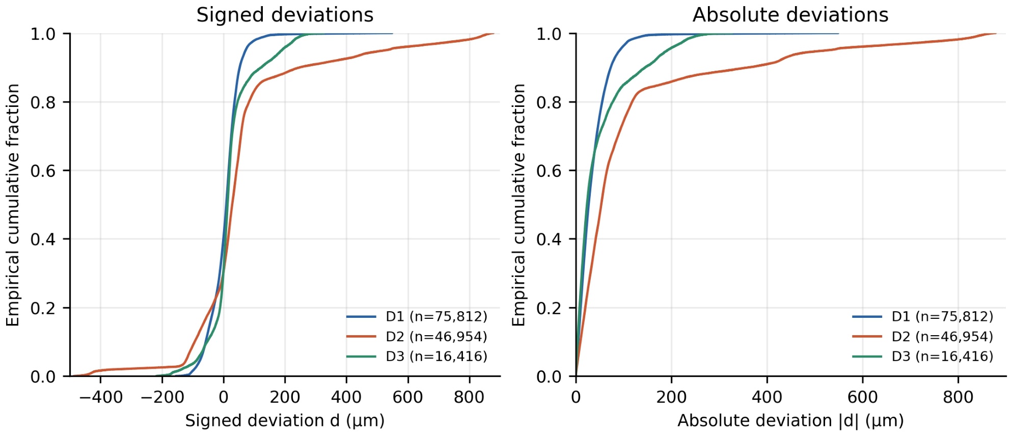
Fig. 5.
Vertex-based ECDFs of signed μCT-to-CAD nearest-surface deviations d (left) and absolute deviations |d| (right). The three curves use complete but differently meshed component surfaces.
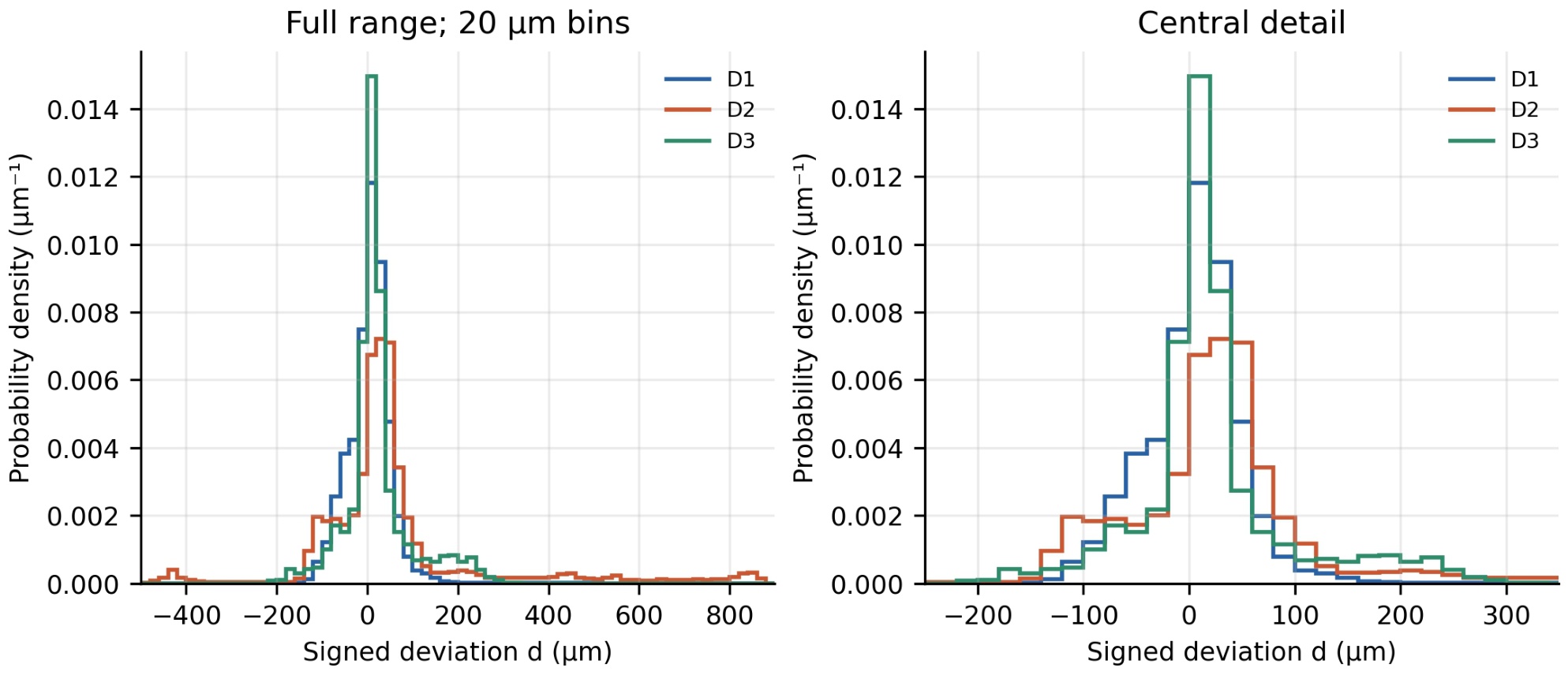
Fig. 6.
Histograms of signed vertex deviations normalized to probability density (μm−1). The entire range (left) and central detail (right) use identical 20 μm bins and density values. Each full histogram has unit area.
Table 2 gives 100G̑j(Δ) at selected diagnostic widths. At 20 μm, D3 covers 44.17% of its vertices, more than D1 (38.60%). D1 has higher coverage at 50 μm and every wider reported band. D2 has the lowest coverage at each threshold. This change in ordering between D1 and D3 illustrates why central concentration and upper tails should be shown together. These are fractions of mesh vertices; they are not area fractions or toleranced pass rates.
B. Normality diagnostics and parametric approximation
Table 3 reports additional diagnostics for the same complete signed vertex exports as Table 1. All three distributions are positively skewed and have positive excess kurtosis, most prominently D1 in the latter measure. The fitted-normal AD statistics are 795.21, 4414.05, and 833.92 for D1, D2, and D3, respectively. The conventional independent-observation AD calculation returns p ≤ 0.0005 (its lower reporting bound) for each component. This nominal result is consistent with the visible departures from a Gaussian shape, but its usual inferential calibration does not apply to spatially correlated vertices.
Table 3.
Normality diagnostics and exploratory marginal fits for the full signed vertex-deviation exports.
| Quantity | D1 | D2 | D3 |
|---|---|---|---|
| N | 75 812 | 46 954 | 16 416 |
| Skewness | 1.34 | 1.88 | 0.88 |
| Excess kurtosis | 12.05 | 5.56 | 2.37 |
| AD statistic (normal) | 795.21 | 4414.05 | 833.92 |
| Nominal AD p | ≤ 0.0005 | ≤ 0.0005 | ≤ 0.0005 |
| AIC (normal) | −242577 | −18493 | −39028 |
| AIC (Student’s t) | −255007 | −62871 | −46548 |
The location-scale Student’s t fit has a lower AIC than the normal fit for each component. The improvement is descriptive evidence that allowing heavier symmetric tails better represents these vertexwise marginals than a normal density. It does not establish that a Student’s t model adequately reproduces their positive skewness or spatially localized extremes, nor does it validate draws from that fit for uncertainty propagation.
C. Pairwise empirical-distribution comparisons
Table 4 presents the maximum vertical differences between the component ECDFs. For the signed deviations, the KS distance is 0.2474 for D1–D2, 0.1111 for D1–D3, and 0.2092 for D2–D3. Comparing absolute deviations gives 0.2908, 0.1175, and 0.2878, respectively. The signed and absolute comparisons answer different questions: a positive and negative departure of the same magnitude contribute differently to F̑ but identically to G̑.
Table 4.
Pairwise maximum distances between the vertex ECDFs of the three individual components.
| Component pair | DKS(d) | DKS(|d|) |
|---|---|---|
| D1–D2 | 0.2474 | 0.2908 |
| D1–D3 | 0.1111 | 0.1175 |
| D2–D3 | 0.2092 | 0.2878 |
Table 4 contains the observed distances only. Their magnitudes indicate how far the empirical vertex distributions separate on the displayed scale; they have no sampling-based significance interpretation for a population of parts. The three different components are each represented by one reconstructed mesh, so vertices cannot be treated as independent production replicates.
D. Spatial structure within D1
The 12 D1 axial intervals contain exactly its 75 812 exported vertices. Count-weighted pooling reconstructs the global mean and RMS in Table 1, confirming consistency between the global and regional computations. Their common width is 1.013 mm over the observed y range −0.036 to 12.119 mm. Fig. 7 shows that the largest bin RMS, 81.18 μm, occurs in interval 6, centered at y = 5.535 mm. Its Q0.95(|d|) is 152.08 μm; the interval contains 6 307 vertices (8.32% of D1).
All 267 D1 vertices with |d| > 200 μm belong to interval 6, including the global extreme. Within a narrower ±100 μm diagnostic band, interval 4 has the lowest coverage (85.22%), whereas interval 6 has the highest (93.82%). The location that requires closer inspection, therefore, depends on the size of the discrepancy of interest. The signed D1 distribution has a descriptive skewness of 1.34 and an excess kurtosis of 12.05. These moments summarize its asymmetric tail and localized extremes; they are not estimates of an underlying independent measurement-error distribution.
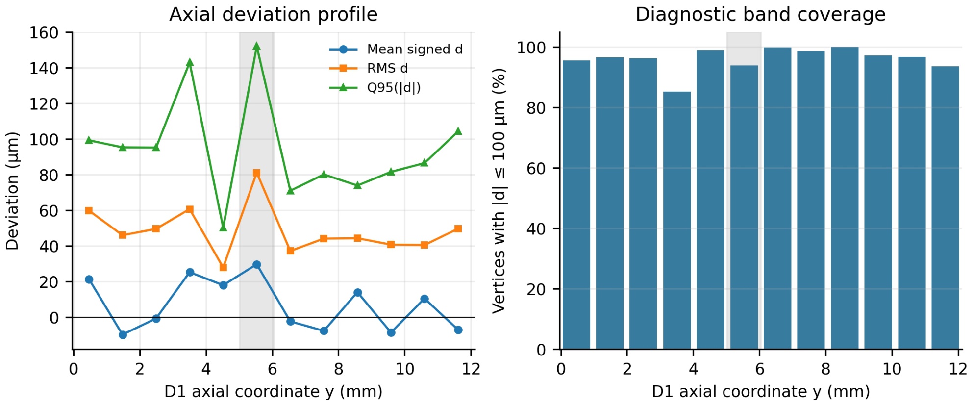
Fig. 7.
Axial analysis of the D1 vertex deviations in 12 equal-width y intervals. Left: signed mean, RMS, and 95th percentile of |d|; right: percentage of vertices with |d| ≤ 100 μm. Shading marks interval 6, which contains every D1 vertex with |d| > 200 μm. Regional weights reflect local mesh density.
Fig. 8 presents an axis-resolved view of D1, where the colored bands indicate uniform intervals along the rotational axis s rather than deviation magnitude. The lower panel shows the regional mean signed radial difference, the radial MAE, and the 95th percentile of the absolute radial difference. Across its 79 841 valid radial values, the supplied statistics give a mean Δr = 27.17 μm, an RMS of 80.49 μm, and Q0.95(|Δr|) = 165.86 μm. Local 95th percentiles can exceed 0.6 mm at around s = −5.25 mm and −3.64 mm; these are sharply localized.
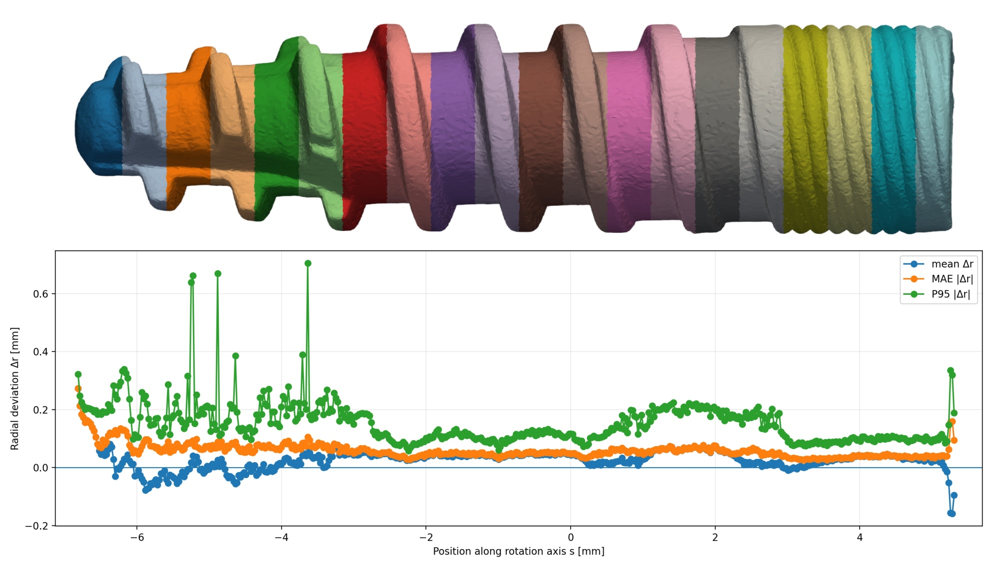
Fig. 8.
Rotational-axis diagnostics of μCT D1 aligned to CAD model. Upper: rendering of 75 812 STL vertices colored by axial region (colors identify regions, not deviation). Lower: 497 intervals along the rotation axis s; signed mean Δr, mean |Δr|, and 95th percentile of |Δr| are computed from 79 841 valid radial locations. The radial difference is defined relative to the recorded axis and must not be equated with the nearest-CAD-surface deviation in Fig. 7.
4. Discussion
The three exported meshes can be compared on a consistent operational basis: the three-component numerical summaries, empirical distributions, and KS distances use their recorded vertex-based signed nearest-surface deviations. D2 has the largest observed broad and tail discrepancies in this representation. The spatial D1 calculation identifies a concentrated region of extreme deviations, even though D1 has the lowest global RMS. The diagnostic ranking of D1 and D3 changes with the chosen bandwidth. These facts demonstrate the value of a distributional and spatial description alongside a global mean.
The spatial density of STL vertices generally varies across the surface and depends on the local triangulation. Consequently, statistics calculated directly from STL vertices are vertex-weighted rather than area-weighted and may over-represent densely triangulated regions, such as threaded or highly curved surface features. Threaded, highly curved, or otherwise densely meshed regions may receive disproportionate weight. The separately supplied 80 000 area-sampled D1 CAD-normal differences provide a useful check: their mean is 7.71 μm, RMS 47.54 μm, Q0.95(|d|) = 92.86 μm, and fraction with |d| ≤ 50 μm is 77.78%, versus 5.22 μm, 49.14 μm, 92.08 μm, and 75.89% for the 75 812 vertex-based nearest-surface differences. The two D1 summaries are numerically close but describe different sampling measures and different geometric projections; the differences cannot be attributed solely to mesh density. Area sampling reduces the influence of uneven tessellation when its uniformity is checked, at the cost of a separate sampling algorithm and its coverage and correspondence choices. Vertex analysis preserves the supplied STL sites and straightforward localization on that mesh, but gives dense mesh regions extra weight. A controlled comparison would calculate both nearest-surface and normal deviations at the same area-sampled points, assess edge cases, and examine the results by functional region.
The evaluated (investigated) components have different geometries, and each is represented by one mesh; the pairwise ECDF distances should be read alongside the plots to identify where their vertexwise distributions differ; they cannot isolate a manufacturing-process effect. The separate radial D1 analysis highlights another consequence of measurand choice: radial ray differences on threads with multiple intersections can have much larger local percentiles than signed nearest-surface distances. Its axis and intersection rule should be checked against the relevant datum and mating geometry before using radial profiles to modify a manufacturing operation.
A parametric representation may be useful for future tolerance simulations, provided the model is chosen for a specified surface, sampling measure, and geometric deviation definition. A skew-normal distribution can represent asymmetry, a Student’s t distribution can represent symmetric heavy tails, and a finite mixture may describe distinct surface regions or multiple modes; these alternatives would require graphical and tail-quantile checks against the ECDF and spatial maps before use. In particular, a fitted vertexwise distribution does not by itself supply a joint spatial model or a distribution of manufactured parts. A generalized extreme-value model would require defined block maxima, whereas a generalized Pareto model could be considered for exceedances above a justified high threshold. Neither tail framework is estimated from the present data. The empirical vertex distributions remain the primary descriptions in this study.
The integrated descriptive workflow combines explicitly defined vertex deviations, empirical distributions, and spatial diagnostics for three individual μCT-derived implant components. In the vertex analysis, D2 has the largest RMS and upper absolute-deviation tail, while D1’s largest outliers are confined to a specific axial interval. Separate D1 sampling and radial outputs show why the geometric definition and correspondence must accompany each reported summary. The observation model identifies calibration, acquisition, surface determination, and registration as contributors to a feature-specific uncertainty budget. These findings can prioritize inspection of the examined components; further uncertainty assessment, as well as conformity and process-capability evaluation, require the additional measurements and definitions described above.
5. Conclusion
This study developed and evaluated an automated metrological and statistical workflow covering the complete chain from μCT acquisition and surface reconstruction through CAD registration to the determination, statistical characterization, and spatial evaluation of geometric quantities. The workflow was applied to three geometrically different components forming a dental implant assembly, representing different challenges for μCT-to-CAD evaluation: a geometrically complex surface, substantial deviations from the nominal CAD geometry, and an ambiguous initial orientation requiring robust global registration.
The automated coarse-to-fine registration reduces operator dependence and improves robustness when local differences between the measured surface and the CAD model are large, such as in the case of the D2 component. The D3 case demonstrates the importance of global registration, as its omission can lead to gross rotational misregistration. In our study, the differences between the resulting statistical summaries were small relative to the registration uncertainty when a sufficient number of alignment points was used. The Monte Carlo analysis also provided an estimate of registration uncertainty that should be considered when evaluating the uncertainty of the selected dimensions.
The statistical and spatial analyses further demonstrate that the measurement result depends on the definition of the measurand, spatial sampling, and geometric correspondence. Signed nearest-surface, CAD-normal projection, and radial deviations, therefore, represent different geometric measurands and may lead to different statistical characteristics. Combining empirical statistical distributions with spatially resolved analysis enables the distinction between broadly distributed discrepancies and localized geometric deviations that may be obscured by global statistical parameters.
The complete workflow provides a reproducible basis for the metrological and statistical evaluation of dimensional and geometric parameters while reducing contributions associated with manual processing and registration. Together with μCT acquisition and surface determination, registration, and geometric-parameter estimation, the statistical evaluation provides a basis for assessing the measurement uncertainty of a selected dimensional and/or geometric quantity. Together, these methods offer a way to examine contributions arising from CT measurement, registration, and the determination of geometric parameters relevant to the manufacture of three representative dental implant components. They also provide a basis for repeatable measurements of the same parameters across manufactured components and their subsequent statistical evaluation.
Acknowledgment
This work was supported by the Recovery and Resilience Plan of the Slovak Republic under project DigiDent No. 09I05-03-V02-00080, “Research on the Digitalization of Dental Implant Components for the Creation of Personalized 3D Models for Manufacturing Processes.”
Notes
[5] Data and reproducibility
The main analyses use component-specific vertex-deviation datasets. Supplementary D1 area-sampled, rotational-region, and ray-based datasets are identified separately in the Methods and Results. The accompanying MATLAB program calculates descriptive statistics, ECDFs, density-normalized histograms, KS comparisons, and D1 axial summaries from the vertex datasets, as well as selected statistics from the D1 metrology and radial workbooks. Supplementary MATLAB code reproduces the fitted-normal AD diagnostic with stable log-tail evaluation, and the exploratory normal and Student’s t fits from the full D1–D3 signed vertex exports. The accompanying results table records the diagnostic statistics and information criteria; the fitted models are not calibrated uncertainty distributions. Raw μCT volumes, complete CAD and measured STL meshes, and repeated scans are held by the authors for further analysis and verification; the present numerical results were derived from the tabular exports. Full reproduction of acquisition and reconstruction additionally requires the original projection data and documented scanner settings. Reproduction of surface extraction requires the segmentation convention and its software implementation. Reproduction of registration would require access to the manufacturer-controlled CAD revisions, identified reference features and datums, alignment transformations, and complete best-fit settings, which are not released in the present tabular dataset. The proprietary CAD revision identifiers are retained in project records but are not published.