
1. Introduction
High-ohm resistors are used in precise picoammeters when measuring very low currents. Picoammeters often use a so-called feedback ammeter circuit that includes an operational amplifier and a high-resistance resistor in the feedback loop [1]. In this circuit, the operational amplifier must exhibit high accuracy and a very low input noise current [2]. Precise picoammeters are used, for example, to measure the concentration of air ions [3], [4], the relative permittivity of building materials [5], or the electrostatic field [6].
When measuring very low currents, it is crucial to minimize low-frequency noise. The noise level limits the minimum measurable level. The randomness of a noise signal only concerns its instantaneous amplitude, while the statistical properties of noise are time-independent [7]. Noise occurs in all electronic circuits, regardless of the components used or their connections. Due to the random nature of noise signals, the mean noise power, the mean quadrature voltage or the mean quadrature current are most commonly used to describe them. Due to the variability in noise power (voltage or current) across frequency bands, the term noise spectral power density (voltage or current) was introduced, referring to a bandwidth of 1 Hz [8]. In electronic circuits, two types of noise are generated, which are distinguished by their frequency dependence. White noise is characterized by a uniform distribution of frequency components in the spectrum. The second type of noise is colored noise, which is characterized by a non-uniform spectral distribution.
The most important of the white noises for us is Johnson’s thermal noise. It occurs in conductors and semiconductors and is generated by both active and passive components. It is generated by the movement of electrons at temperatures above 0 K. Its spectral power density can be considered constant up to a frequency of 100 THz: at higher frequencies, other types of noise start to appear, and the spectral power density takes an increasing trend. The approximate effective value of the noise voltage on a resistor due to Johnson’s thermal noise is given by:
where kB is the Boltzmann constant (kB = 1.380·10−23 J·K−1), T is the absolute temperature of the resistor in Kelvin, R is the resistance of the resistor and BN is the considered noise.Equation 1 shows that the square of the noise voltage increases with the resistance of the resistor. Thermal noise from the real resistive parts of all impedance types appears in the circuits. When measuring voltage, the magnitude of Johnson’s thermal noise is determined by the internal resistance of the sample, whereas when measuring current, it is necessary to consider Johnson’s thermal noise due to the internal resistance of both the measured sample and the measuring device [1].
Reducing the noise bandwidth BWN can effectively reduce the mean value of noise voltage or current. The bandwidth BW of useful signals is defined as a 3 dB drop from the maximum voltage or current magnitude. However, noise bandwidth BWN is defined differently. It is determined based on the equality of the total noise power at the output of the selective circuit and the equivalent noise power that we would obtain at the output of a bandpass filter with ideal rectangular transfer characteristics [7]. According to this definition, the area under the black curve in Fig. 1 is equal to the area of the blue rectangle, and it is clear that the noise bandwidth is greater than the bandwidth for a 3 dB drop.
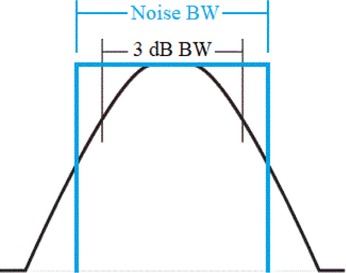
Fig. 1.
Noise bandwidth determination.
Another type of noise to consider when measuring very small DC voltages and currents is 1/f flicker noise. In some literature [9], [10], it is referred to as current noise because it is proportional to the flowing current. Resistors made using thick-film technology generate 1/f flicker noise at a level significantly higher than resistors made using thin-film technology. The spectral density of flicker noise can be expressed as a function of voltage drop across a resistor [9]. With a higher voltage drop, the spectral density of flicker noise increases. In articles [11], [12], [13], and [14], the generation and modeling of 1/f flicker noise in semiconductors are investigated and discussed.
Paper [15] discusses using the low-frequency noise of thick-film resistors as an indicator of their quality and reliability. According to this article, resistors made with silver as the conductive material show more significant changes in noise and resistance in some cases.
The Wheatstone bridge allows precise measurement of resistance and small resistance changes; however, the circuit is also regularly applied to measure resistor noise, as shown in [16], where thick-film resistor properties were measured depending on temperature. Connecting the Wheatstone bridge requires four resistors of an identical series and resistance values. Unfortunately, the tolerance of the measured resistor results in a DC offset at the input of the differential amplifier, limiting the amplification. Instrumentation operation electrometer amplifiers for high-ohm measurements are not widely available at present, and the regularly obtained parameters are generally inferior to those of a classic operational amplifier. An adverse aspect also rests in the need for four resistors, with good quality models being expensive to purchase.
When designing more accurate methods for measuring low-frequency noise in high-ohm resistors, we have to employ a connection that substitutes the instrumentation amplifier with a precise electrometer operational amplifier. Another requirement, then, is to reduce the number of measured resistors. Further, the proposed measuring technique is expected to eliminate or effectively decrease the noise in the measuring system. Common methods for measuring up to 1 MΩ with only one resistor require a separating low-noise resistor, usually a wound manganese-based resistor, and, given the high values of the measured resistances, the technique (mentioned in the MIL-STD-202 standard) is unsuitable.
The central aim of this article is to design and verify the functionality of a system for measuring the low-frequency noise of high-ohm resistors, namely, a system that eliminates the drawbacks of the method that applies the Wheatstone bridge.
Second, a prominent objective within the above goal is to compare the resistor manufacturing technologies, above all, the metal-oxide and thick-film technologies, the latter exploiting low voltages. This procedure also involves confirming the hypothesis that metal-oxide resistors generate a very low level of 1/f flicker noise and are suitable for use in precise picoammeters or current-to-voltage converters.
Another related task is to determine the impact of voltage loss and housing on excessive 1/f flicker noise in thick-film resistors. Table 1 lists the resistors tested in the experiments presented herein, including their parameters.
Table 1.
The tested resistors and their parameters.
| Resistor technology | Metal-oxide | Thick-film | Thick-film |
|---|---|---|---|
| Resistance [GΩ] | 1 | 1 | 1 |
| Tolerance [%] | ±1 | ±1 | ±1 |
| Manufacturer | Ohmite | Ohmite | Ohmite |
| Series | RX-1M Hi-Meg | Slim-Mox | Maxi-Mox |
| Number | RX-1M1007FE | SM102031007FE | MOX-1-121007FE |
| Package | Glass sealed | Planar | Axial |
| Rated voltage [kV] | 1 | 5 | 10 |
| Thermal coefficient [PPM/°C] | 50 | 25 | 100 |
| VCR voltage coefficient [PPM/V] | - | < 5 | < 2 |
| Number of tested samples | 2 | 10 | 1 |
2. Measurement Setup
A more accurate setup for measuring low-frequency noise in thick-film resistors can advantageously utilize the circuit from article [17], Fig. 2. This connection uses only two tested resistors, compared to the Wheatstone bridge approach, which requires four. The measured resistor noise is the average noise between the two resistors. The difference in the values of the two resistors will again appear as a DC offset in the measured voltage, similarly to the Wheatstone bridge. Thus, the tolerance of the applied resistors again restricts the maximum amplification of the first amplifier in the cascade. A major benefit is that we do not need an instrumentation amplifier, as the measured effect at the common node of the measured resistors is the voltage to earth, not the differential voltage.
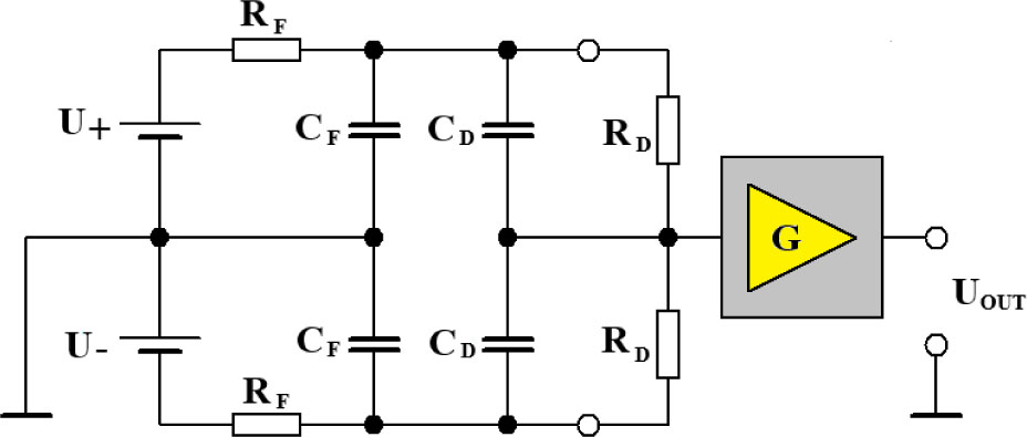
Fig. 2.
The circuit diagram for measuring resistor 1/f flicker noise with two identical resistors [17].
In this circuit, two symmetrical voltage sources, U+ and U−, must supply the same voltage. The resistors RF and capacitors CF represent a low-pass filter. The resistors RD are two measured resistors, and the capacitors CD represent their parasitic capacitance. The measured resistors and their parasitic capacities together form a low-pass filter, reducing the measured bandwidth. At higher resistor values, the measurable bandwidth decreases. Now, active shielding is required because the resistors need to be placed in a shielding case, and additional capacitance would further reduce the bandwidth. The improvement achieved through active shielding was measured on the setup.
To eliminate or effectively reduce the measuring system noise, the circuit in Fig. 2 is suitable; moreover, corrections are feasible based on the properties of the non-correlable noise in the measured sample and the background noise of the measuring system, as described in [18]. The authors of the article state that it is possible to easily measure the noise of the measured sample if its level is at least 10 dB (3x) higher than the background noise of the measuring system. If this condition cannot be met, it is advisable to use two channels of the spectrum analyzer and their correlation as shown in Fig. 3.
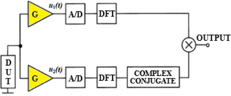
Fig. 3.
The block diagram for noise measurement using the correlation of two channels of a spectrum analyzer [18].
This approach uses two low-noise operational amplifiers connected after the measured resistors. Subsequently, a discrete Fourier transform is performed on both channels of the spectrum analyzer, and mathematical operations are used to compute the correlation of the spectra of the signals at the output of both operational amplifiers. The noise generated by the operational amplifiers in the circuit is largely eliminated in this way because it is uncorrelated, unlike the noise of the measured resistors.
Using the principles established in previous studies, Fig. 2 and Fig. 3, we can develop a method to measure the 1/f flicker noise of high-ohm resistors [19]; the accuracy of the procedure is expected to surpass that of the classic connection based on the Wheatstone bridge. Active shielding then allows measuring the noise properties up to the higher frequencies.
The circuit is shown in Fig. 4. The two voltage sources from Fig. 2 were replaced by one voltage source and two low-noise operational amplifiers, one for each channel. One amplifier is in an inverting configuration and the other is in a non-inverting configuration. Their gain should be equal to one. To the outputs UA and UB, a differentiator with a cut-off frequency of 0.1 Hz is connected, separating the DC component; then, we connect the input of a spectrum analyzer, facilitating mutual correlation and representation of the measured values.
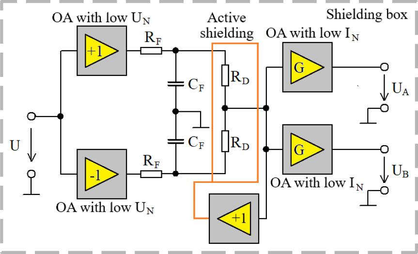
Fig. 4.
The circuit diagram for measuring resistor 1/f noise with two identical resistors and two channels of a spectrum analyzer [19].
3. Measured Results with New Equipment
According to the diagram in Fig. 4, the measurements were made with two identical resistors. We measured two metal-oxide and two thick-film resistors of the Slim-Mox 102 series. The parameters of the measured resistors are presented in Table 1. The voltage applied to the resistors was 4.9 V in both cases. The power supply was from batteries, and the resistors were enclosed in a shielding case that was actively shielded using a buffer [1], [19]. The voltage drop on the resistors was achieved using two OPA211 precision operational amplifiers, which have very low input noise voltage. To amplify the output noise voltage of the resistors, LMC6001A operational amplifiers with a very low input noise current and current offset were used. Their gain was 40 dB. The manufacturer of the LMC6001A operational amplifier specifies the noise input current of 0.13 fA/√Hz at a frequency of 1 kHz. A photo of the measuring equipment in the shielding box is shown in Fig. 5.
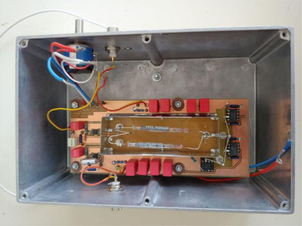
Fig. 5.
A photo of the measuring equipment in the shielding box.
Table 2.
The changes in the upper cut-off frequency in relation to the measured resistor.
| Resistor | Frequency [Hz] | |
|---|---|---|
| No active shielding | Active shielding | |
| 10 MΩ | 5500 | 6880 |
| 100 MΩ | 677 | 840 |
| 1 GΩ | 68 | 93 |
| 10 GΩ | 6.5 | 9.5 |
| 100 GΩ | 0.95 | 1.54 |
| 500 GΩ | 0.27 | 0.45 |
| 1 TΩ | 0.19 | 0.37 |
The spectral noise voltage density was measured in two frequency bands for both types of resistors by means of a HP 35660A spectrum analyzer. The lower frequency band was from 0.3 Hz to 25 Hz, and the higher frequency band was from 10 Hz to 100 Hz. The averaging was performed from one hundred readings in both frequency bands. The measured effective values at the input of the spectrum analyzer in dBVrms were converted to the spectral noise voltage density of the resistors in μV/√Hz. The conversion had to be calculated separately for each frequency band. For the measurement, we selected a uniform FFT window (uniform ENBW = 1, Hannig ENBW = 1.5, flat-top ENBW = 3.81). First, the bandwidth was converted to the decibel measure:
Subsequently, the effective value at the input of the spectrum analyzer in dBVrms was converted to the spectral density in dBV/√Hz by subtracting the decibel measure bandwidth from the measured values:
Then, we determined the spectral density by subtracting the operational amplifier’s amplification in the decibel measure from the spectral density at the input of the analyzer. After that, the spectral density at the input of the amplifier LMC6001A was converted to the absolute measure in V/√Hz by delogarithmization:
The computation also had to be performed for the measured noise background values to facilitate correction. The diagram in Fig. 6 exposes the spectral density of the input noise voltage at short-circuiting the input and relates to both input channels. Similarly, the input noise current was measured when a metal-oxide 500 GΩ resistor had been connected to the input. These two data items characterize the measurable noise threshold of the equipment. The correction was performed by subtracting the square of the measured noise from the square of the input noise voltage and the input noise current multiplied by the magnitude of the resistor being measured:
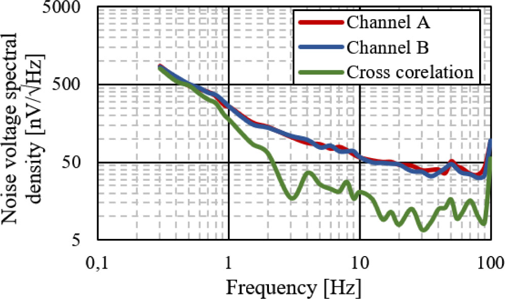
Fig. 6.
The spectral input noise voltage of the measuring system for the resistor noise measurements.
Cross-correlation enabled us to reduce the input noise voltage three times, while no improvement was observed in the input noise current. Thus, cross-correlation decreases the measurement uncertainty, especially for the lower values of the measured resistors.
The resulting calculated value indicates the spectral density of the noise voltage of the parallel combination in the measured resistors in V/√Hz. Within the last step, the values were converted to μV/√Hz. Since the noise voltage spectral density was measured across two resistors, at the last stage, we had to multiply the values by √2 to match the theoretical level of a single resistor with a magnitude of 1 GΩ.
Next, we calculated the necessary correction for various magnitudes of the measured resistors related to frequency. In Microcap, we simulated the bandwidth of the measured noise voltage at the output of the designed equipment (Fig. 7), assuming the manufacturer-specified resistor capacitance of 0.7 pF; this value was then additionally verified with an Instek LCR 6004 RLC meter. Further, we measured a 1 GΩ resistor with and without active shielding. At low frequencies, the differentiator, C = 100 μF and R = 22 kΩ, is applied, separating the DC component at the output of the measuring equipment. The limiting factor that restricted the bandwidth at high frequencies proved to be the capacitance of the measured resistor, a property that cannot be further reduced. By contrast, the capacitance to the shielding case can be effectively reduced via active shielding. The value of 1.2 pF was established by combining measurement with a Microcap simulation. Without active shielding, the usability of measurement at high resistor values, namely those above 500 GΩ, would be markedly restricted; at such levels, we would already be operating outside the working range of the designed setup.
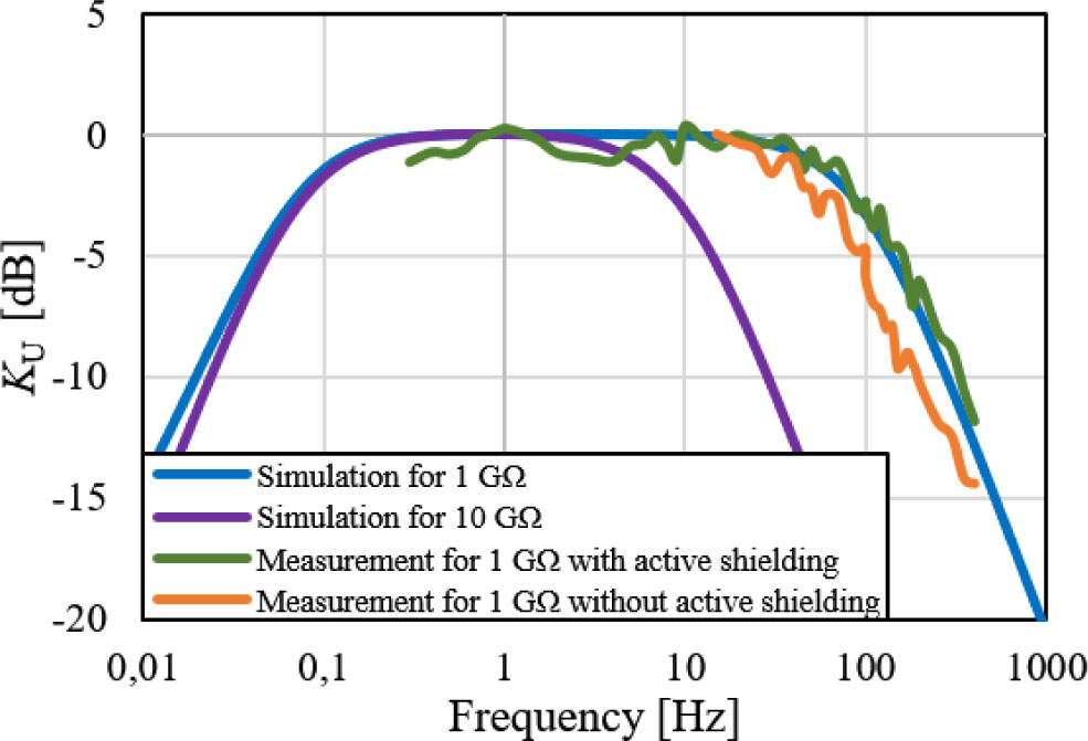
Fig. 7.
The simulated and the measured frequency characteristics of the measuring setup with and without active shielding.
Next, we computed the difference between the noise value measured with the designed setup and the theoretical value of the resistor thermal noise in Table 3. With the higher resistor values, the measurement cannot be performed at the higher frequencies. However, an inverse-function-based correction is applicable, depending on whether we know the resistor’s parasitic capacitance exactly.
Table 3.
The standard deviation for the measured resistor noise spectral density without cross correlation.
| Frequency [Hz] | 0.3 | 0.5 | 1 | 5 | 10 | 50 | 100 |
|---|---|---|---|---|---|---|---|
| Noise voltage [nV/√Hz] | 857 | 475 | 251 | 84 | 57 | 46 | 51 |
| Noise current [fA/√Hz] | 0.09 | 0.09 | 0.09 | 0.09 | 0.09 | 0.09 | 0.09 |
| Resistor | Deviation [%] | ||||||
| 10 MΩ | 216 | 94 | 33 | 4 | 2 | 1 | 2 |
| 100 MΩ | 38 | 13 | 4 | 0 | 0 | 0 | 0 |
| 1 GΩ | 4 | 1 | 0 | 0 | 0 | 0 | 0 |
| 10 GΩ | 1 | 1 | 0 | 0 | 0 | - | - |
| 100 GΩ | 4 | 4 | 4 | - | - | - | - |
| 500 GΩ | 20 | 20 | - | - | - | - | - |
| 1 TΩ | 37 | - | - | - | - | - | - |
Fig. 8 shows the noise voltage spectral density for a pair of metal-oxide resistors and a pair of resistors made by thick-film technology. For thick-film Slim-Mox resistors, a high increase in spectral density at low frequencies due to 1/f flicker noise is visible. The noise of the metal-oxide resistors can be considered constant over the entire measured band. At the lowest measured frequency of 0.3 Hz, the noise of the thick-film resistors is twice as high as the noise of the metal-oxide resistors, even though the Slim-Mox series are very high-quality thick-film resistors. In the figure, the theoretical level of Johnson’s thermal white noise for a 1 GΩ resistor is also plotted, calculated using (1).
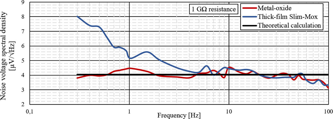
Fig. 8.
Measured noise voltage spectral density of metal-oxide and thick-film Slim-Mox series resistors.
In the white noise range, the measured noise voltage spectral density corresponds to approximately 4 μV/√Hz. For a resistance of 1 GΩ, the spectral noise current density is calculated to be 4 fA/√Hz. According to the manufacturer, the operational amplifiers LMC6001A used to amplify the measured noise have the input noise current spectral density of 0.13 fA/√Hz. The measured noise current of the resistors is approximately forty times higher than the input noise current of the operational amplifiers. The signal-to-noise ratio, therefore, corresponds to approximately 32 dB.
At higher frequencies, the decrease in spectral density is caused by the attenuation of a low-pass filter, consisting of measured resistors and their parasitic capacitance, as shown in the circuit diagram in Fig. 2 and the upper cutoff frequency in Table 2.
To verify the effect of the applied voltage on the resistor’s 1/f noise, measurements were performed for voltages of 0 V, 2 V, 3 V, and 4.9 V. As shown in Fig. 9, 1/f noise increases with voltage loss. Without applied voltage, the noise from a thick-film resistor is equal to thermal noise. This fact is important, for example, when designing a current-to-voltage converter, where it is not advantageous to fully utilize the operational amplifier’s output voltage swing, and it is better to choose a lower voltage loss. For example, when measuring air ions, excessive noise can compromise the processing of results for the saturation characteristics.
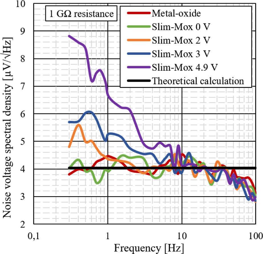
Fig. 9.
Measured spectral voltage density as a function of the voltage drop across the measured resistor.
Oscilloscope display with time courses of the output of both channels (green and yellow) and their difference (pink) is in Fig. 10.
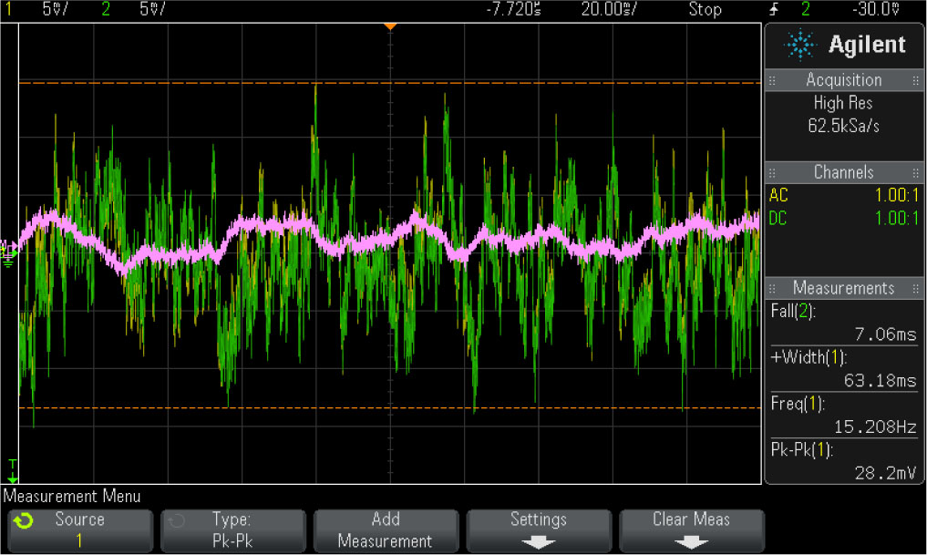
Fig. 10.
Time course of resistor noise voltage for both channels (yellow and green) and their difference (pink).
4. Measured Results with Electrometer
The resistance dependence on the applied voltage was also measured for both resistors. The measurements were performed using a 6517A electrometer from Keithley Instruments. Using a built-in voltage source, the applied voltage was adjusted, and the current through the resistors was measured. We measured 50,000 current values at each voltage level. The sampling was controlled by a program in the VEE environment. Considering the long measurement time and the large number of measured values, we processed only one metal-oxide and one thick-film resistor from the Slim-Mox series in Table 1. The relationship between resistance and voltage loss was then computed from the measured time courses (Fig. 11). In the image, the crosses represent the mean value of the resistance, determined from the entire time courses of the current. The standard deviations of resistance are listed in Table 4.
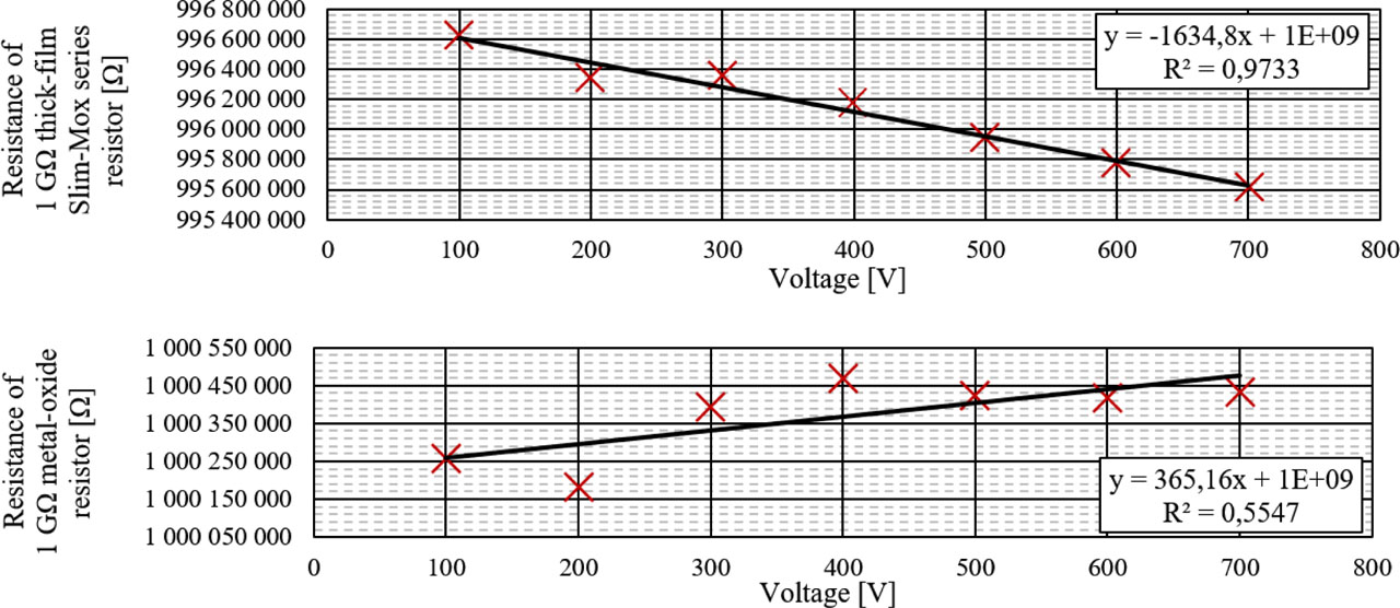
Fig. 11.
Resistance dependence on the applied voltage for a 1 GΩ thick-film Slim-Mox series resistor and a 1 GΩ metal-oxide resistor.
Table 4.
Standard deviation for measured resistance dependence on the applied voltage.
| Voltage [V] | 100 | 200 | 300 | 400 | 500 | 600 | 700 |
|---|---|---|---|---|---|---|---|
| Metal-oxide [kΩ] | 58.8 | 16.1 | 10.6 | 7.4 | 6.3 | 5.8 | 6.8 |
| Slim-Mox [kΩ] | 4.8 | 2.5 | 12.7 | 10.8 | 11.6 | 11.1 | 14.1 |
During the measurement, the resistors were enclosed in a shielding vessel and located on Teflon spacers to reduce the effect of leakage currents. Both resistors exhibit a manufacturer-specified value tolerance of ±1 %. In these resistors, the most prominent deviation of the mean value of the measured resistance from the nominal value of 1 GΩ appeared at a resistor voltage loss of 700 V. The deviation of a Slim-Mox thick-film resistor corresponds to a resistor value decrease of 0.46 %, while in a metal-oxide resistor the value increase deviation amounts to only 0.055 %.
According to Table 1, the metal-oxide resistor is rated for 1 kV, and the Slim-Mox thick-film resistor is rated for 5 kV. The current flowing through the resistors at the applied voltages was very low. The temperature in the laboratory remained constant throughout the measurement. The temperature coefficient of a metal-oxide resistor is 50 PPM/°C, and the temperature coefficient of the Slim-Mox resistor is 25 PPM/°C. The slope of the line used to interpolate the measured mean values in Fig. 11 should not be assigned to temperature stability, but rather to voltage stability. The voltage coefficient of a Slim-Mox resistor eventually equaled −1.635·10−6 V−1, with the corresponding value in the metal-oxide resistor being 0.035·10−6 V−1.
The authors of article [9] present an option for expressing the relationship between the magnitude of the noise voltage spectral density and the magnitude of the voltage loss on the resistor. This relationship is measurable with an electrometer. In a 6517A electrometer, the maximum sampling speed is 15 samples per second. With a sufficiently long sampling time, this approach allows measuring frequencies lower than those processible by using the spectrum analyzer. The control window in the VEE environment is shown in Fig. 12.
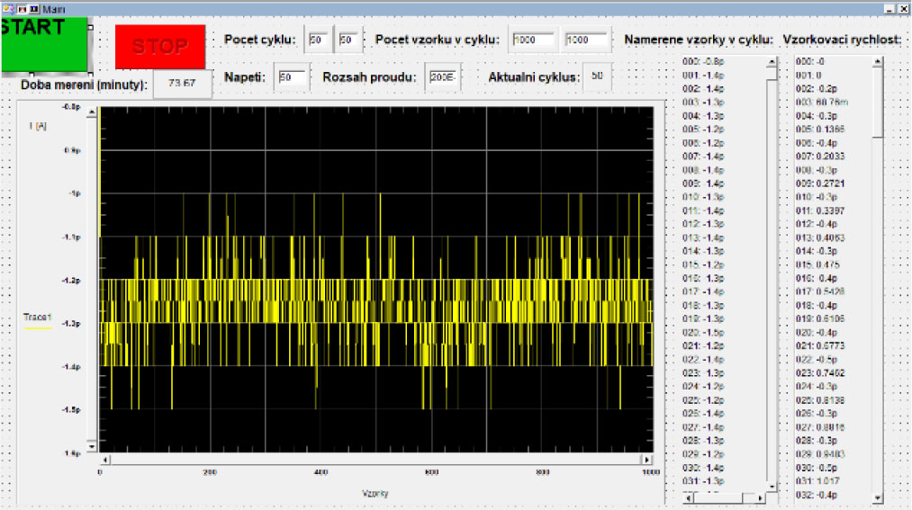
Fig. 12.
The main screen of the resistor current sampling application in the VEE environment.
The obtained time dependences of the current through the resistor had to be further converted to the noise current spectral density using Matlab. This step involved, first of all, removing the DC component, which was eliminated via subtracting the moving average of the measured values with an averaging period of 1000 samples from the measured values, according to (7).
Subsequently, we used the Matlab functions in the form:
where ABS is a Matlab function that computes the absolute value, FFT is a function computing the discrete Fourier transform by means of an algorithm for the Fast Fourier transform, and N is the Fourier transform length of 50 thousand samples. As only the unilateral spectrum was computed, the entire computation had to be multiplied by two and then divided by the square root of N. In the last step, the spectral density was again averaged using a moving average with a sampling period of 100 samples.To make fit also the horizontal axis for the unilateral spectrum, we had to convert the number of samples to a frequency, as shown by the Matlab notation:
where f is the frequency on the horizontal axis, fs denotes the sampling frequency of 15 Hz, and N stands for the Fourier transform length of 50 thousand samples. The frequency resolution is 0.1 mHz.The measured dependence of the voltage noise spectral density is due to a voltage loss on the resistor between 4.9 V and 190 V. For higher voltage loss values, the input range of the electrometer would need to be increased. The voltage noise spectral densities of the thick-film resistors were determined only within an electrometer input range of up to 200 pA. The sampling again invariably included 50 thousand samples per hour, with the measured resistors enclosed in a shielding vessel and located on Teflon spacers. The measuring station is shown in Fig. 13.
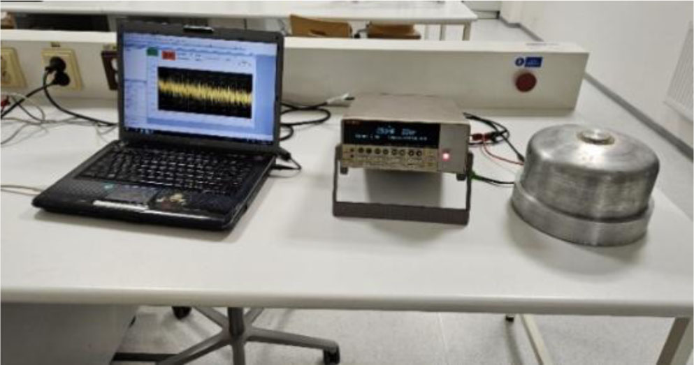
Fig. 13.
The measuring station with the Keithley 6517A electrometer.
First of all, we measured the noise current spectral density of a metal-oxide resistor, for which a very low level of 1/f flicker noise had been observed in our previous measurement. The background noise current spectral density for each acquired voltage loss on the resistor was established through subtracting the theoretical noise current spectral density level on the 1 GΩ resistor from the values obtained on the metal-oxide resistor (10):
Next, we focused on the noise current spectral density of the electrometer’s actual low-noise input, with the voltage source disconnected and observing the given input range. The measured noise current spectral densities for each voltage loss on the resistor, with the voltage source disconnected, are presented in Fig. 14. The figure shows that the noise of the actual low-noise input of the electrometer is negligible. With the voltage source connected, the spectral density exhibits a rowth at lower frequencies. The electrometer is supplied from the grid, making it possible that the higher noise in the electrometer’s voltage source is generated by the switched circuits and filters in the feeding segment of the electrometer.
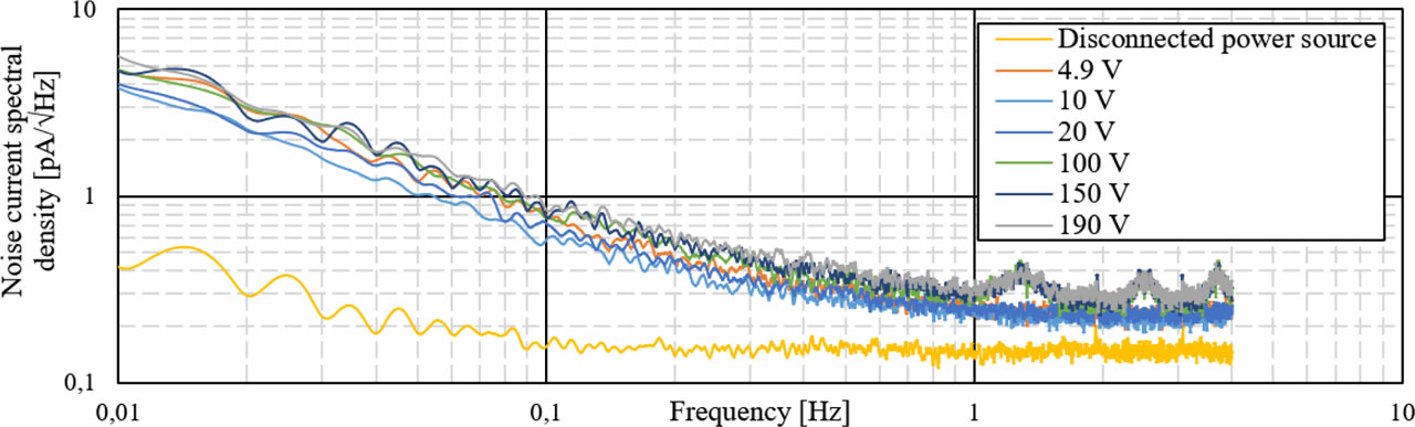
Fig. 14.
The 6517A electrometer background noise current spectral density.
Further, we determined the noise current spectral density in the two thick-film resistors. One of these two items, a Slim-Mox resistor, had a slim case; the other, a Maxi-Mox, had a larger, round case. The resistor’s parameters are characterized in Table 1. We measured only one resistor of each type because the measurements are time-intensive.
The obtained noise current spectral densities were corrected by subtracting the noise current spectral densities of the voltage source from Fig. 14, see (11):
In the thick-film resistors, we measured noise current spectral densities that were an order of magnitude higher than those of the voltage source.
Next, we converted the noise current spectral density to the noise voltage spectral density by multiplying the resistor 1 GΩ value according to (12):
The last correction task consisted of averaging the noise voltage spectral density, with a moving average period of 700 samples. In this context, Fig. 15 shows the noise voltage spectral density computed from the values measured for the Slim-Mox series thick-film resistor, and Fig. 16 shows the noise voltage spectral density obtained from the measured values for the Maxi-Mox series thick-film resistor. Due to averaging, the noise voltage spectral densities are reliable only above 0.04 Hz.
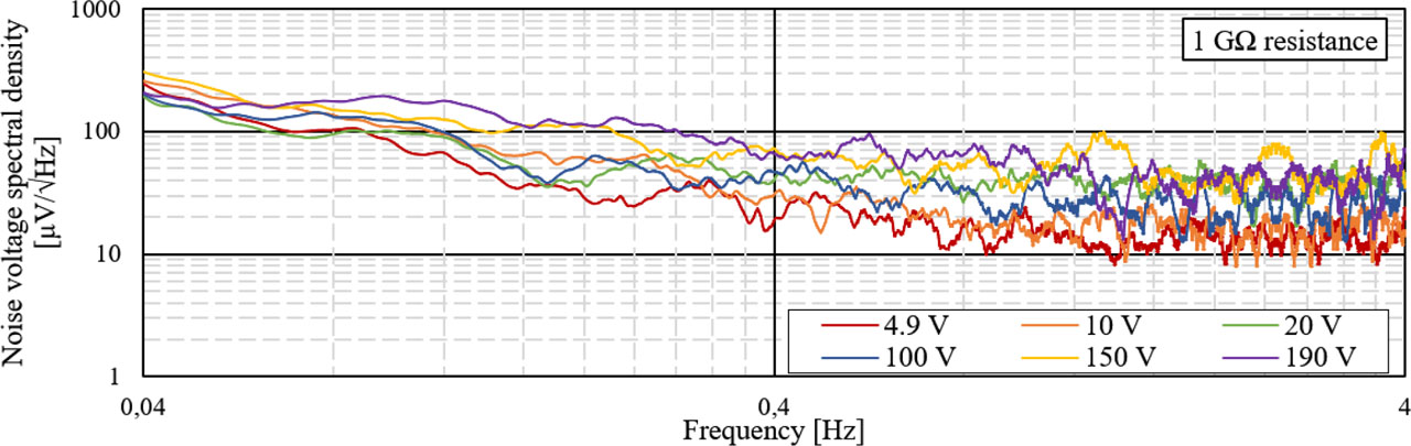
Fig. 15.
Noise voltage spectral density measured using the 6517A electrometer for a 1 GΩ thick-film Slim-Mox series resistor.
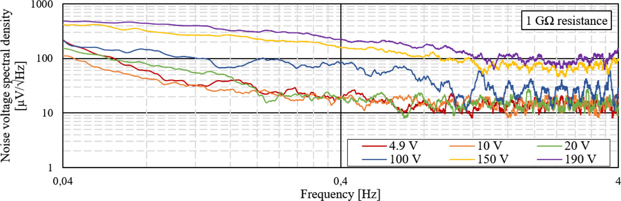
Fig. 16.
Noise voltage spectral density measured using the 6517A electrometer for a 1 GΩ thick-film Maxi-Mox series resistor.
The measurement confirmed that the noise voltage spectral density increases with increasing voltage loss on the resistor. For the voltage loss of 4.9 V on the Slim-Mox series resistor, the voltage noise spectral density in the white noise domain ranges between 10 μV/√Hz and 20 μV/√Hz. The theoretical noise voltage spectral density of the 1 GΩ resistor, according to (1), is 4.0 μV/√Hz. The benefit of using an electrometer to measure the noise voltage spectral density is the ability to determine higher voltage losses in a simple manner.
To compare the voltage noise spectral densities for both thick-film resistor types, we can point to the Maxi-Mox resistor exhibiting a stronger relationship between the noise voltage spectral density and the voltage loss on the resistor. Further, in this branch of measurement the resistors did not exhibit major heating. Thus, the difference between the resistors with respect to the above-noted relationship cannot be attributed to their thermal dependence or to heating during the measurement.
For each resistor, we computed the voltage coefficients from the measured current time courses; the relevant values are 1.4·10−6 V−1 for the Slim-Mox resistor and 2·10−6 V−1 for the Maxi-Mox resistor. According to the manufacturer’s specifications in Table 1, the Slim-Mox and the Maxi-Mox resistor’s voltage coefficients should be below 5 PPM/V and 2 PPM/V, respectively. Based on the measured data, we can conclude that the Slim-Mox thick-film resistor features a lower voltage coefficient value than its Maxi-Mox counterpart. The manufacturer-specified limits have been met by both resistors.
5. Measurement of a Set of Thick-Film Resistors
To verify the repeatability of the measurements, the voltage coefficient of ten resistors was measured at voltages of 700 V and 100 V. Pairs of resistors with similar voltage coefficients were then selected, and their noise was measured using the proposed equipment with a spectrum analyzer at a frequency of 0.3 Hz (Table 5). The results indicate good repeatability. The resistors are from the same series, so there is minimal variation in both parameters.
Table 5.
Verification of the repeatability of the voltage coefficient (VCR) and noise measurements for a series of Slim-Mox resistors.
| Resistor samples | Tolerance [%] | VCR [PPM/V] | Noise [µV/√Hz] |
|---|---|---|---|
| 1 | –0.43 | –5.29 | 8.8 |
| 2 | –0.33 | –3.84 | |
| 3 | –0.54 | –3.49 | 8.6 |
| 5 | –0.23 | –3.90 | |
| 8 | –0.64 | –4.59 | 8.3 |
| 10 | –0.65 | –5.07 | |
| 4 | –0.61 | –4.03 | 8.1 |
| 9 | –0.18 | –4.04 | |
| 6 | –0.44 | –4.16 | 7.9 |
| 7 | –0.15 | –4.11 |
6. Discussion
The noise-voltage spectral characteristics measured via the spectrometer method suggest that the metal-oxide resistor generates a virtually negligible level of 1/f low-frequency noise. When determining the relationship between the resistance values and the voltage losses in the resistors, we observed that the metal-oxide resistor had a resistance value very close to the nominal value of 1 GΩ across all the measured voltages. Thus, the metal-oxide resistor was used as the reference item throughout the measurements.
Interestingly, in the white-noise domain, the electrometer-measured noise-voltage spectral density in the thick-film resistors exceeded the computed theoretical level by approximately tenfold. According to the explanatory hypothesis, this deviation arises from the electrometer-voltage-source noise, which cannot be adequately eliminated by subtraction from the values measured with the thick-film resistors. The noise background spectral density was found to be an order of magnitude lower than the noise voltage spectral density with the resistors, meaning that merely subtracting the values does not yield sufficient correction; the electrometer voltage source noise will then invariably manifest itself in the values measured with the thick-film resistors. This hypothesis is verifiable if an external voltage source with a very low noise level can be used.
The Maxi-Mox thick-film resistor shows a stronger relationship between the noise-voltage spectral density and the voltage loss than its Slim-Mox counterpart. This fact results from several factors that need to be considered at various degrees of possibility and importance: differences in housing size and shape, manufacturing discrepancies, and resistor voltage coefficient. Based on computations from the measured values, the Maxi-Mox resistor voltage coefficient is higher than that of the Slim-Mox component. Thus, the voltage coefficient depends on the relationship between the noise voltage spectral density and the voltage loss. To confirm the hypothesis, we would need to measure more resistors, comparing a much wider range of factors and aspects.
7. Conclusion
The research in this article used previous methods to develop a novel setup for measuring noise in high-ohm resistors. This newly designed approach eliminates the drawbacks of the Wheatstone bridge-based technique, measuring average noise with only two resistors and without requiring an instrumentation amplifier. The setup also employs the principle of mutual correlation between two spectrum analyzer channels, which can reduce background noise by as much as 10 dB. The measured noise results in high-ohm resistors within white noise almost match the theoretical values. Mutual correlation is especially advantageous when the resistance of the measured resistors is below 100 MΩ. At high resistance values, due to their parasitic capacitance, the bandwidth and the maximum measurable frequency nevertheless decrease. The measured bandwidth corresponds to the theoretical one obtained from computer simulations. The bandwidth was successfully extended thanks to active shielding, an outcome important for resistances of high values.
Further, the innovated procedure described in this article allowed confirming experimentally the hypothesis that a metal-oxide resistor generates very little 1/f flicker noise, whereas the Slim-Mox thick-film resistors produce such noise at a nonnegligible level. Using electrometer measurements, we found that a metal-oxide resistor is also more accurate in its resistance value and features a lower voltage coefficient than the Slim-Mox series resistors. A metal-oxide resistor is therefore more suitable for use in precise current-to-voltage converters and picoammeters.
The final chapters of the article discuss using an electrometer to compare the spectral noise voltages of two thick-film resistors from the Slim-Mox and Maxi-Mox series. Applying an electrometer enables us to measure even with higher voltage losses across the resistor; however, the results are not as precise as those obtainable with the spectrum analyzer method. The acquired data indicate that a thick-film Maxi-Mox resistor shows a stronger dependence of the noise-voltage spectral density on the resistor voltage loss. This resistor also exhibits a higher voltage coefficient. However, further measurements are needed to determine whether the dependence between the noise-voltage spectral density and the resistor voltage loss is generated or influenced by the resistor voltage coefficient, the housing shape, or the actual inner structure of the resistor.
Acknowledgment
The research was completed with support from the project No. FEKT-S-23-8425, which was supervised by the BUT internal grant office.