

Figure 1
Relationship between CM and CBB.
Source: Authors’ own research.
Table 1
NCA feature selection.
Table 2
The algorithm steps of kNN.
| 1 | Determine the value of , |
| 2 | Calculate the distance between the new instance and the entire training set , |
| 3 | Determine the nearest neighbors by sorting the distances from smallest to largest, |
| 4 | Determine the class of the new instance by majority voting. |
Source: Authors’ own research results.
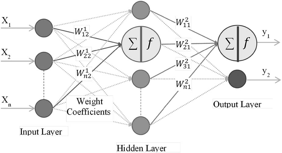
Figure 2
Neural network model.
Source: Authors’ own research results based on Neural Networks.
Table 3
The algorithm steps of ELMs.
| 1 | Assign weights and biases randomly |
| 2 | Calculate hidden layer output, H |
| 3 | Calculate output weight matrix , |
| 4 | Use to predict the classes of testing data |
Source: Authors’ own research results based on ELM.
Table 4
Sample distribution table of the subjects participating in the study.
| Variables | Frequency (f) | Percent (%) | |
|---|---|---|---|
| Gender | Female | 180 | 47.6 |
| Male | 198 | 52.4 | |
| Age | 17–18 | 16 | 4.2 |
| 19–20 | 177 | 46.8 | |
| 21–22 | 137 | 36.2 | |
| 23–24 | 33 | 8.7 | |
| 25 and more | 15 | 4.0 | |
| Body type | Slim | 92 | 24.3 |
| Normal | 237 | 62.7 | |
| Large | 49 | 13.0 | |
| Educational level | Associate degree | 299 | 79.1 |
| Bachelor’s degree | 79 | 20.9 | |
| Science field | Social sciences | 324 | 85.7 |
| Science | 36 | 9.5 | |
| Health Sciences | 18 | 4.8 | |
| Level of income | 1,000 TL and less | 224 | 59.3 |
| 2,000 TL | 85 | 22.5 | |
| 3,000 TL | 24 | 6.3 | |
| 4,000 TL | 11 | 2.9 | |
| 5,000 TL and more | 34 | 9.0 | |
| Total | 378 | 100 | |
Source: Authors’ own research.
Table 5
Distribution table of socio-demographic characteristics of the subjects participating in the study.
| Variables | Frequency (f) | Percent (%) | |
|---|---|---|---|
| Relationship (partner) | Yes | 132 | 34.9 |
| No | 246 | 65.1 | |
| Place of birth | Big city | 171 | 45.2 |
| Province | 99 | 26.2 | |
| County | 99 | 26.2 | |
| Village | 9 | 2.4 | |
| Living place | Big city | 243 | 64.3 |
| Province | 79 | 20.9 | |
| County | 46 | 12.2 | |
| Village | 10 | 2.6 | |
| Mother’s education level | Illiterate | 23 | 6.1 |
| Primary school | 156 | 41.3 | |
| Secondary education | 156 | 41.3 | |
| University | 43 | 11.4 | |
| Father’s education level | Illiterate | 8 | 2.1 |
| Primary school | 137 | 36.2 | |
| Secondary education | 162 | 42.9 | |
| University | 71 | 18.8 | |
| State of illness | Yes | 48 | 12.7 |
| No | 330 | 87.3 | |
| Total | 378 | 100 | |
Source: Authors’ own research.
Table 6
Cronbach’s alpha test.
| Scale | Number of expression | Cronbach alpha |
|---|---|---|
| CM | 4 | 0.823 |
| CBB | 11 | 0.792 |
Source: Authors’ own research.
Table 7
Kmo–Bartlett’s test.
| Kaiser–Meyer–Olkin measure of sampling adequacy | 0.835 | |
| Bartlett’s test of sphericity | Approx. chi-square | 5174.812 |
| df | 435 | |
| Sig. | 0.000 | |
Source: Authors’ own research.
Table 8
Exploratory factor analysis.
| Factor 1 | Factor 2 | ||
|---|---|---|---|
| CM Cr. Alpha = 0.823 | Get experience with tattooing | 0.618 | |
| Desire to join a community | 0.847 | ||
| Socialization or group interaction | 0.902 | ||
| Social differentiation | 0.846 | ||
| CBB Cr. alpha = 0.792 | Do you have a tattoo? | 0.441 | |
| Would you like to get a tattoo? | 0.701 | ||
| What are the reasons why you don’t want to get a tattoo? | 0.650 | ||
| Do you want to get a permanent tattoo or a temporary tattoo? | 0.897 | ||
| On which part(s) of your body did you have your tattoo done or would you like to have it done? | 0.599 | ||
| Does anyone in your family have a tattoo? | 0.850 | ||
| Do any of your friends have tattoos? | 0.875 |
Source: Authors’ own research.
Table 9
Goodness of fit indexes of scales.
| Scale model | ΔX 2 | sd | p | ΔX 2/sd | GFI | CFI | RMSEA | RMR |
|---|---|---|---|---|---|---|---|---|
| CM | 7.274 | 6 | 0.06 | 1.21 | 0.85 | 0.97 | 0.03 | 0.04 |
| CBB | 5.489 | 3 | .23 | 1.83 | 0.89 | 0.95 | 0.04 | 0.02 |
Notes: (i) The relationship is significant at the p < 0.01 significance level (ii) ΔX 2 (chi-square test result of cm, sd (degrees of freedom), p (significance value), ΔX 2/sd (chi-square value of cm divided by degrees of freedom), GFI (absolute fit index), CFI and RMSEA (comparative fit index) , RMR (residual based fit index).
Source: Authors’ own research.
Table 10
Model fit criteria goodness of fit index reference ranges.
| Model fit criteria | Good fit | Acceptable fit |
|---|---|---|
| X 2 Uyum Testi | 0.05 < p ≤ 1 | 0.01 < p ≤ 0.05 |
| CMIN/SD | X 2/sd ≤ 3 | X 2/sd ≤ 5 |
| Comparative fit indexes | ||
| CFI | 0.97 ≤ CFI | 0.95 ≤ CFI |
| RMSEA | RMSEA ≤ 0.05 | RMSEA ≤ 0.08 |
| Absolute fit indexes | ||
| GFI | 0.90 ≤ GFI | 0.85 ≤ GFI |
| Residual compliance indexes | ||
| RMR | 0 < RMR ≤ 0.05 | 0 < RMR ≤ 0.08 |
Source: Authors’ own research.
Table 11
Correlation analysis results.
| Measurement data | 1 | 2 |
| 1. CM | 1 | |
| 2. CBB | 0.315** | 1 |
Notes: (i) **At p < 0.01 significance level, the relationship is significant (Spearman rho).
Source: Authors’ own research.
Table 12
Chi-Square analysis results among CBB categories.
| Would you like to get a tattoo? | |||||
|---|---|---|---|---|---|
| Yes | No | Total | |||
| Did you get a tattoo? | Yes, I did | Frequency | 213 | 8 | 221 |
| Did you get a tattoo? | 96.4% | 3.6% | 100.0% | ||
| Would you like to get a tattoo? | 29.3% | 1.3% | 16.5% | ||
| No, I did not | Frequency | 514 | 604 | 1,118 | |
| Did you get a tattoo? | 46.0% | 54.0% | 100.0% | ||
| Would you like to get a tattoo? | 70.7% | 98.7% | 83.5% | ||
| Total | Frequency | 727 | 612 | 1,339 | |
| Did you get a tattoo? | 54.3% | 45.7% | 100.0% | ||
| Would you like to get a tattoo? | 100.0% | 100.0% | 100.0% | ||
Notes: (i) Pearson Chi-Square X 2 = 188.920, p = 0.000 (ii) At p < 0.01 significance, the relationship is significant.
Source: Authors’ own research.
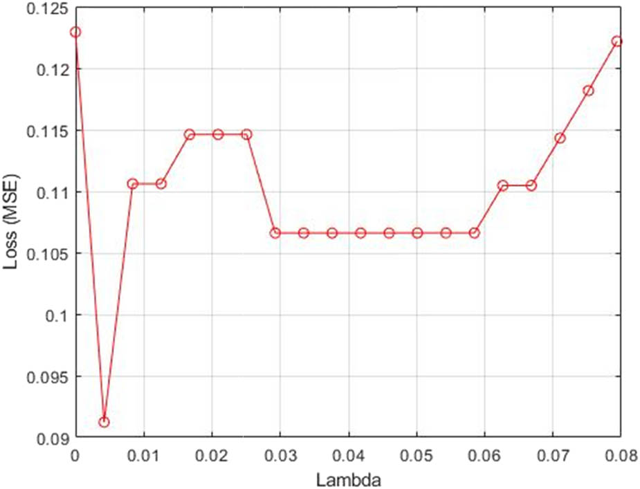
Figure 3
Loss values versus the λ values.
Source: Authors’ own research results.
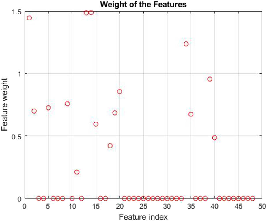
Figure 4
Weight of the features.
Source: Authors’ own research results.
Table 13
Prediction with all features.
| Method* | Accuracy | Specificity | Precision | Recall | F-Measure |
|---|---|---|---|---|---|
| KNN | 89.77 | 87.33 | 89.26 | 91.64 | 90.27 |
| SVM | 87.54 | 85.46 | 87.49 | 88.72 | 87.84 |
| ELM | 87.32 | 81.48 | 85.49 | 91.60 | 88.23 |
Notes: (1)* Parameters of Learning Algorithms: KNN with k = 1, 3, 5, 7. SVM with Kernel RBF and Polynomial, Order = 2, 3, 4, 5. ELM: Activation Function is Sigmoid, Number of Hidden Neurons 10, 20, 30, 40, 50.
Source: Authors’ own research results.
Table 14
Prediction with selected features by using NCFS.
| Method* | Accuracy | Specificity | Precision | Recall | F-Measure |
|---|---|---|---|---|---|
| KNN | 91.02 | 90.98 | 91.91 | 90.51 | 91.03 |
| SVM | 87.63 | 87.14 | 88.46 | 86.91 | 87.47 |
| ELM | 88.54 | 84.98 | 87.29 | 91.34 | 89.13 |
Notes: (1)* Parameters of Learning Algorithms: KNN with k = 1, 3, 5, 7. SVM with Kernel RBF and Polynomial, order = 2, 3, 4, 5. ELM: Activation Function is Sigmoid, Number of Hidden Neurons 10, 20, 30, 40, 50.
Source: Authors’ own research results.