
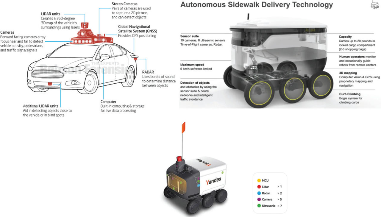
Fig. 1:
Representation of autonomous car and delivery robots with their sensors (Leiss (2018); Kosonen (2020); Lubenets (2021)).
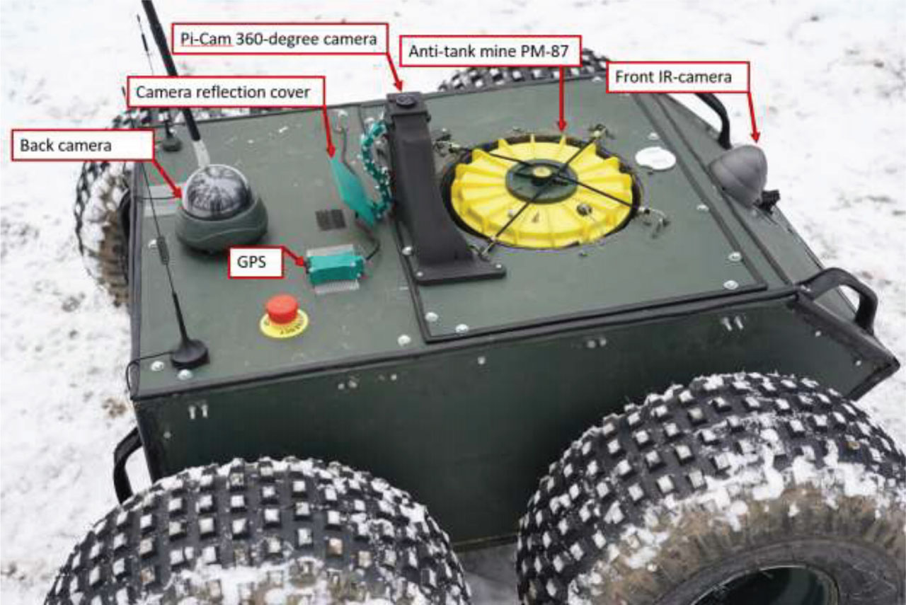
Fig. 2:
Laykka platform with mine-module and 360-degree camera module installed on top.
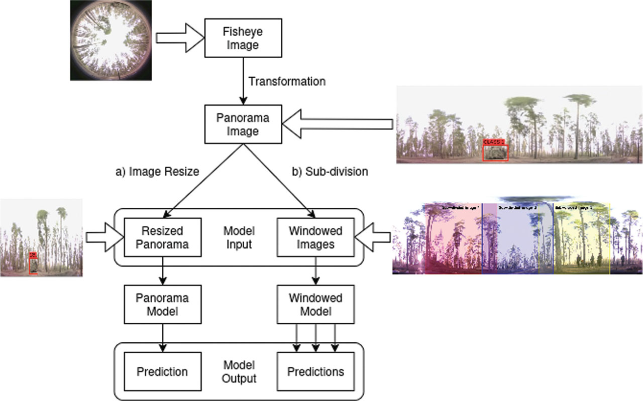
Fig. 3:
Detection framework for converting fisheye images into a panoramic format, followed by model-based inference using one of two alternative configurations. After transformation, the panorama image can either be (a) resized and passed through a Panorama Model for full-image detection, or (b) subdivided into fixed-size windows and processed by a Windowed Model for localised detection. Arrows indicate sequential data flow from image input to prediction output.
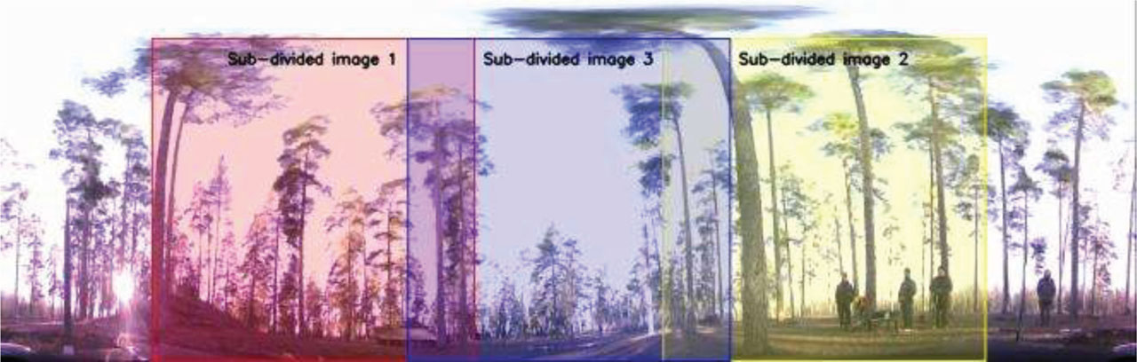
Fig. 4:
The panoramic image is divided into smaller, fixed-size windows to cover the full horizontal field of view. To ensure reliable target detection, the windows are configured with slight horizontal overlap. This overlap allows targets that lie near the edge of one window to still be visible in adjacent windows, reducing the chance of missed detections due to boundary clipping. In practice, this overlapping strategy helps maintain spatial continuity between frames.
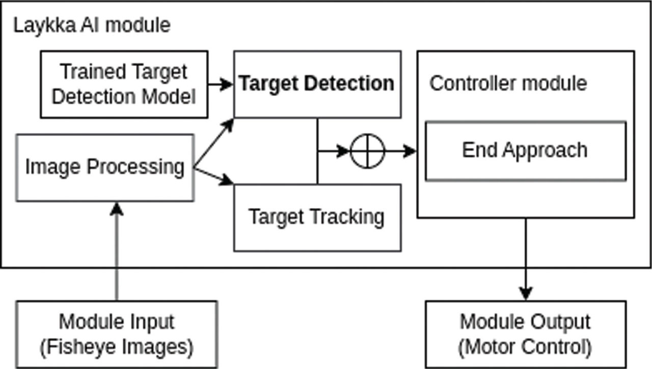
Fig. 5:
Overview of the Laykka AI control module, which integrates object detection and tracking for autonomous decision-making. Arrows indicate data flow: fisheye images undergo preprocessing and detection, feeding into a target tracking component that maintains temporal consistency. These results jointly inform the controller module, which generates motion signals and can trigger an end-approach manoeuvre when conditions are met. The dual-path detection (direct and via tracking) improves robustness in the case of incorrect target detection. AI, artificial intelligence.
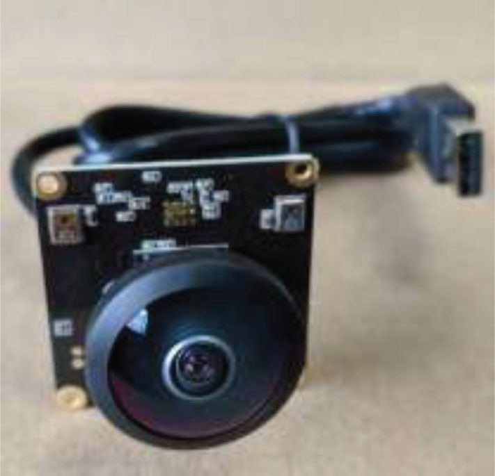
Fig. 6:
PICAM360 camera module (Picam360 Developer Community, P. I 2023). USB-a connector allows for an easy integration with Laykka platform.
Algorithm 1
Object Detection using ML Model
| 1: | Input: Panoramic or windowed image I, previous bounding box Bprev |
| 2: | Output: Detected bounding box Bdet, confidence score Sdet, class label Cdet |
| 3: | Step 1: Load Model and Configuration |
| 4: | Load pretrained object detection model M |
| 5: | Set detection threshold and relevant parameters |
| 6: | Step 2: Prepare Input |
| 7: | Preprocess image I for model input |
| 8: | Step 3: Run Object Detection |
| 9: | Pass image through model: D = M(I) |
| 10: | Extract Bdet, Sdet, and Cdet |
| 11: | Step 4: Filter Predictions |
| 12: | for each detected object do |
| 13: | if confidence score below threshold then |
| 14: | Ignore detection |
| 15: | end if |
| 16: | if Bprev exists then |
| 17: | Compute overlap with previous detection |
| 18: | Define if detection is valid |
| 19: | end if |
| 20: | end for |
| 21: | Step 5: Select Best Detection |
| 22: | Choose highest-confidence valid detection |
| 23: | if no valid detections found then return “no detection” |
| 24: | end if |
| 25: | Return Bdet, Sdet, and Cdet |
Algorithm 2
Fisheye-to-Panorama Transformation (using opencv-python package (cv2) (Rankin 2020; OpenCV Tracker API 2023))
| 1: | Input: Fisheye image Ifisheye of size (Hf, Wf) |
| 2: | Output: Panoramic image Ipanorama of size (Hp, Wp) |
| 3: | Step 1: Compute Mapping Coordinates |
| 4: | procedure BuildMap(Wp, Hp, R, Cx, Cy, offset) |
| 5: | Initialize mapx, mapy ← zero matrices of size (Hp, Wp) |
| 6: | for y ← 0 to Hp − 1 do |
| 7: | for x ← 0 to Wp − 1 do |
| 8: | Compute radius: |
| 9: | Compute angle: |
| 10: | Compute source coordinates: |
| 11: | xs ← Cx + r × sin(θ) |
| 12: | ys ← Cy + r × cos(θ) |
| 13: | mapx[y, x] ← xs |
| 14: | mapy[y, x] ← ys |
| 15: | end for |
| 16: | end for |
| 17: | return mapx, mapy |
| 18: | end procedure |
| 19: | Step 2: Initialize Unwrapper |
| 20: | procedure Initialize Unwrapper(Hf, Wf, Cb, offset) |
| 21: | Cx ← Hf/2, Cy ← Wf/2 |
| 22: | Compute outer radius: R ← Cb − Cx |
| 23: | Compute output image size: |
| 24. | Wp ← ⌊2 × (R/2) × π˼ |
| 25: | Hp ← ⌊R˼ |
| 26: | (mapx, mapy) ← BuildMap(Wp, Hp, R, Cx, Cy, offset) |
| 27: | end procedure |
| 28: | Step 3: Transform Fisheye Image |
| 29: | procedure Unwrap(Ifisheye, mapx, mapy) |
| 30: | i ← cv2.INTER LINEAR |
| 31: | Ipanorama ← cv2.remap(Ifisheye, mapx, mapy, i) |
| 32: | return Ipanorama |
| 33: | end procedure |
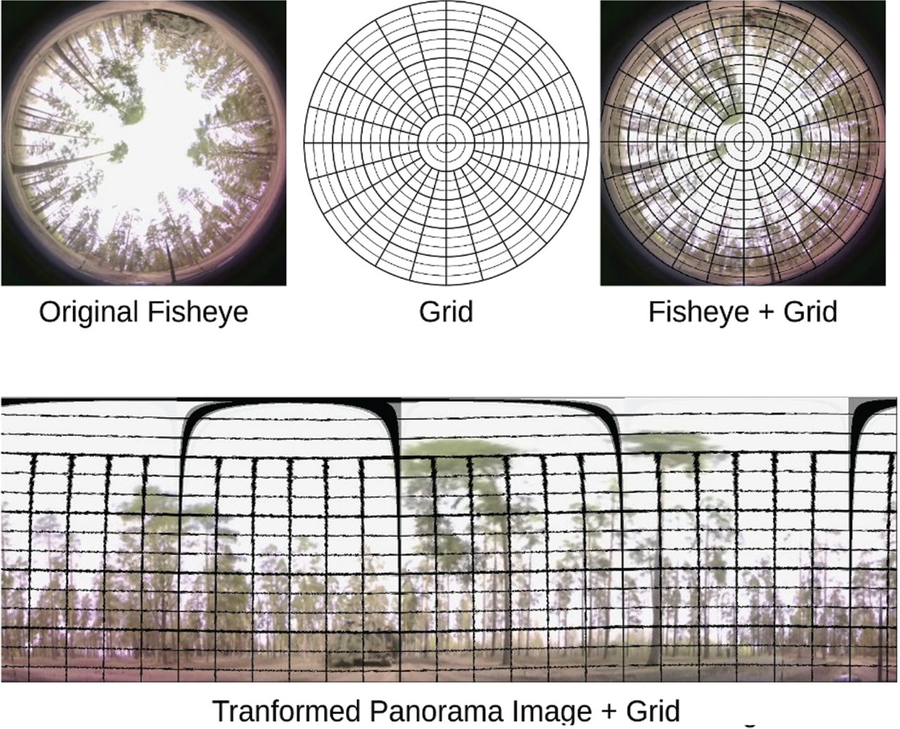
Fig. 7:
Fisheye image transformation visualisation. The grid helps to visualise before and after the transformation.
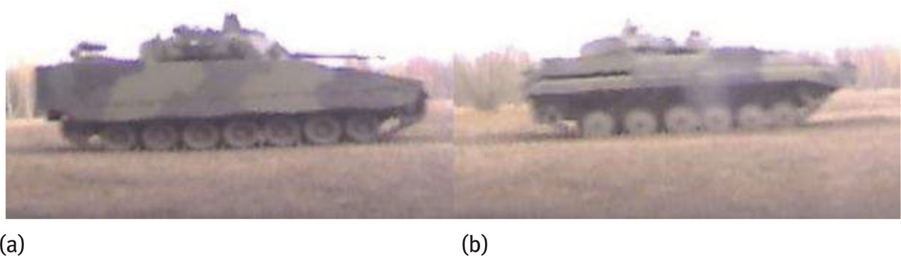
Fig. 8:
Example images of CV90 combat vehicle (a) and BMP-2 combat vehicle (b) classes.
Tab. 1:
Augmentation techniques used in the study
| Technique | Min. value | Max. value |
|---|---|---|
| Random adjust brightness | 0 | 0.5 |
| Random adjust contrast | 0.4 | 1.25 |
| Random adjust saturation | 0.4 | 1.25 |
| Random adjust hue | 0 | 0.01 |
| Random rotation | 0° | 10° |
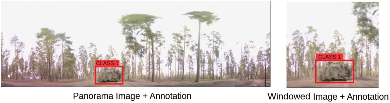
Fig. 9:
Example of two types of the same image used in the training.
Tab. 2:
AP: @0.5 comparison of object detection models on different object sizes, trained on panorama and windowed images (640 × 640 resolution)
| Model | Trained on panorama images | Trained on windowed images | ||||||
|---|---|---|---|---|---|---|---|---|
| APs | APm | APl | AP | APs | APm | APl | AP | |
| SSD ResNet50 V1 | 0.151 | 0.350 | 0.663 | 0.526 | 0.151 | 0.285 | 0.674 | 0.511 |
| Faster R-CNN ResNet50 V1 | 0.101 | 0.243 | 0.661 | 0.471 | 0.151 | 0.268 | 0.667 | 0.501 |
| EfficientDet D1 | 0.000 | 0.197 | 0.588 | 0.402 | 0.151 | 0.418 | 0.692 | 0.567 |
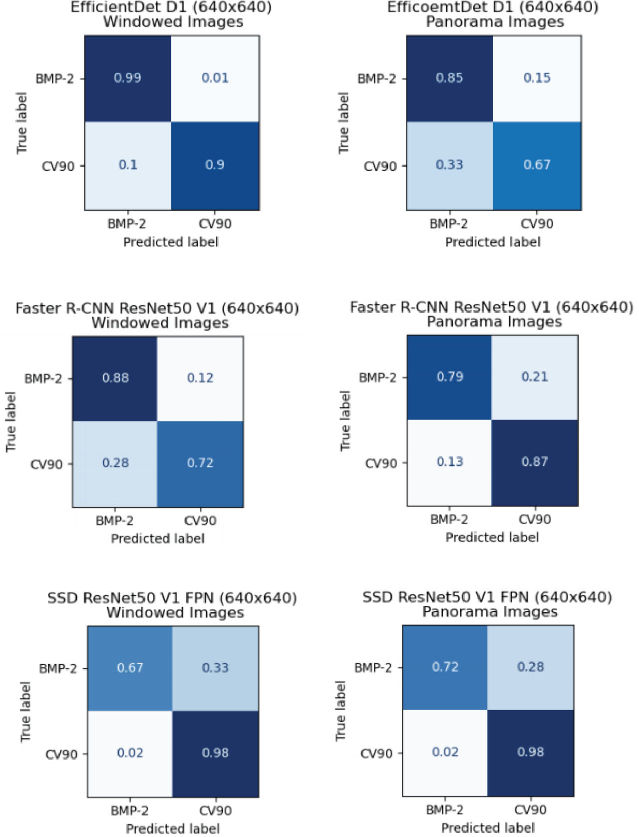
Fig. 10:
A comparison of the models is provided in the form of confusion matrices illustrating the performance of the models on the (left column) windowed and the (right column) panorama image datasets with a resolution of 640 × 640 pixels. Three different models, namely EfficientDet D1, Faster-RCNN ResNet50 V1 and SSD ResNet50 V1 FPN were evaluated. The matrices demonstrate the success rates of distinguishing between the BMP-2 and CV90 classes, with more diagonal values being preferable because they indicate better classification.
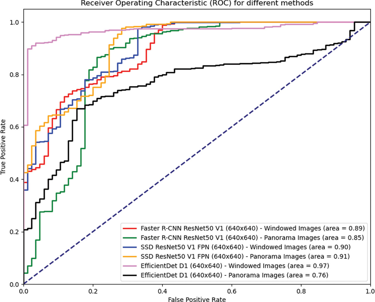
Fig. 11:
ROC curves for object detection models tested on windowed and panorama image datasets at a resolution of 640 × 640. The ROC AUC values indicate comparative performance, with SSD ResNet50 V1 FPN showing the highest consistency and performance across both image types. EfficientDet D1 demonstrates the best performance on windowed images but experiences a notable decline on panorama images. ROC, receiver operating characteristic; AUC, area under the ROC curve.