
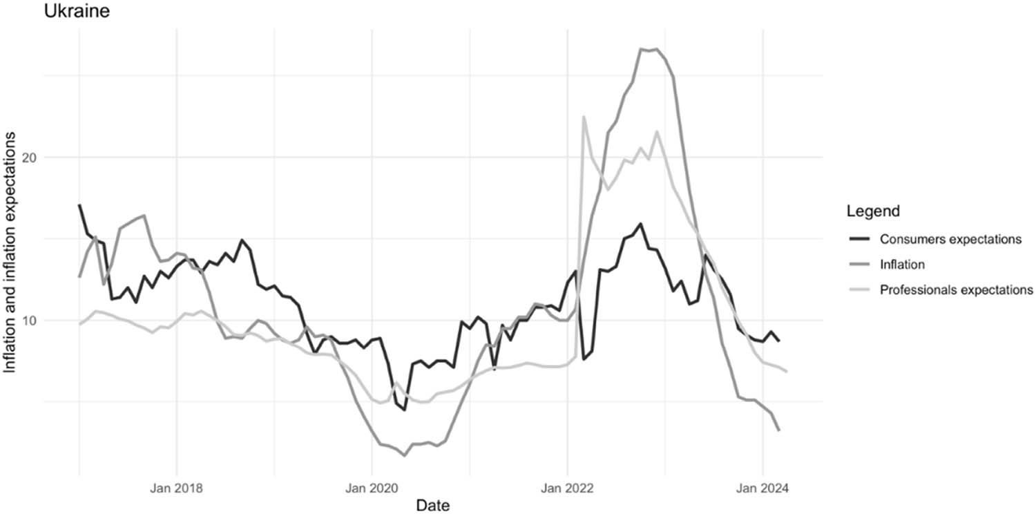
Figure 1
Inflation and expectations in Ukraine.
Source: Consumer expectations: NBU data; professional expectations: Consensus Forecasts of Consensus Economics transformed into fixed horizon forecast by authors; inflation: Ukrstat data.
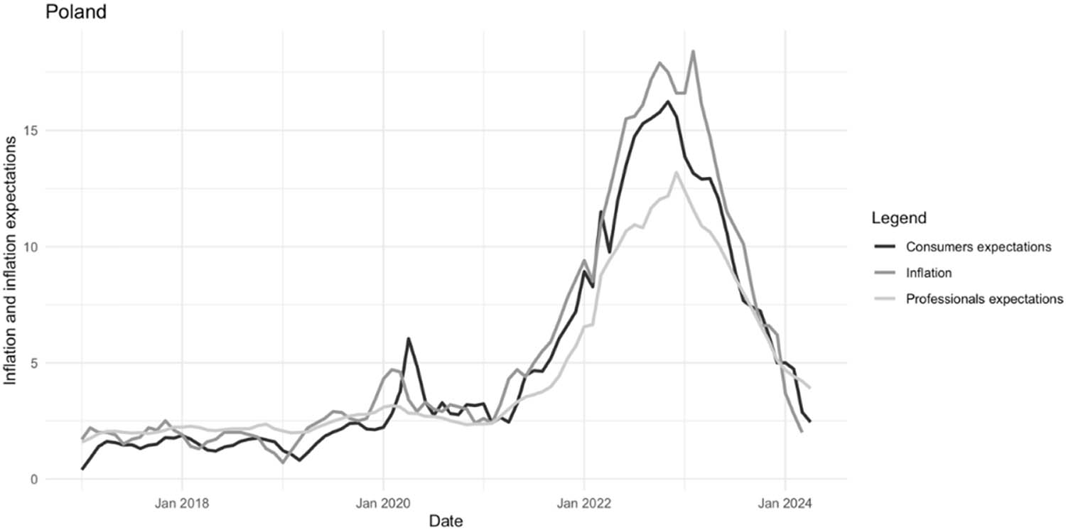
Figure 2
Inflation and expectations in Poland.
Source: Consumer expectations: Business and Consumer Survey, quantified by authors; professional expectations: Consensus Forecasts of Consensus Economics transformed into fixed horizon forecast by authors; inflation: GUS data.
Table 1
Descriptive statistics of stationary differences in inflation and expectations and p-values of the Wilcoxon test and Snedecor–Cochrane F-test for equality of variances before and during the war outbreak.
| Variable | Ukraine | Poland | |||||
|---|---|---|---|---|---|---|---|
| Before | During | p-Value | Before | During | p-Value | ||
| Inflation | Mean | −0.0311 | −0.0300 | 0.0073 | 0.1115 | −0.2600 | 0.0850 |
| SD | 0.9125 | 1.9607 | <0.001 | 0.4673 | 0.2600 | <0.001 | |
| Consumer expectations | Man | −0.0672 | −0.1720 | 0.0157 | 0.1291 | −0.2241 | 0.0196 |
| SD | 1.1763 | 1.8279 | 0.0060 | 0.5762 | 1.2493 | <0.001 | |
| Professional expectations | Mean | −0.0322 | −0.0369 | 0.0001 | 0.0765 | −0.0972 | 0.0247 |
| SD | 0.3329 | 3.1434 | <0.001 | 0.1981 | 0.7512 | 0.0030 | |
Note: p values are for the F test of equality of variances (the null hypothesis is that the variances are equal) and for the Wilcoxon test (the null hypothesis is that the distributions of x and y differ by a location shift of µ; the alternative is that they differ by some other location shift).
Source: Author’s contribution.
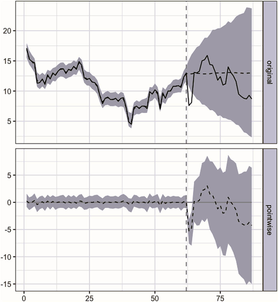
Figure 3
Consumer inflation expectations in Ukraine. Note: During the post-war-outbreak period, the response variable had an average value of approx. 11.79. In the absence of the war, we would have expected an average response of 12.95. The 95% interval of this counterfactual prediction is [6.98, 19.36]. The causal effect (obtained by subtracting the prediction from the response) is −1.16, with a 95% interval of [−7.57, 4.81]. In relative terms, the response variable decreased by −3%. The 95% interval of this percentage is [−39%, +69%]. The probability of obtaining this effect by chance is p = 0.367. This means that the effect may be spurious.
Source: Author’s contribution.
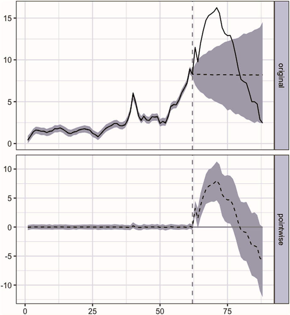
Figure 4
Consumer inflation expectations in Poland. Note: During the post-intervention period, the response variable had an average value of approx. 10.49. In the absence of an intervention, we would have expected an average response of 8.27. The 95% interval of this counterfactual prediction is [4.75, 11.66]. The causal effect (obtained by subtracting the prediction from the response) is 2.22, with a 95% interval of [−1.17, 5.75]. In relative terms, the response variable showed an increase of +33%. The 95% interval of this percentage is [−10%, +121%]. The probability of obtaining this effect by chance is p = 0.091.
Source: Author’s contribution.
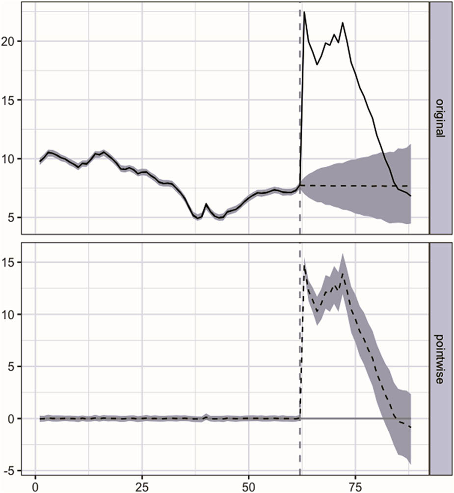
Figure 5
Professional inflation expectations in Ukraine. Note: During the post-war outbreak period, the response variable had an average value of approx. 15.11. In contrast, we would have expected an average response of 7.69 without an intervention. The 95% interval of this counterfactual prediction is [5.66, 9.65]. The causal effect (obtained by subtracting the prediction from the response) is 7.42, with a 95% interval of [5.45, 9.45]. The above results are given in terms of absolute numbers. In relative terms, the response variable showed an increase of +100%. The 95% interval of this percentage is [+56%, +167%]. The probability of obtaining this effect by chance is very small (Bayesian one-sided tail-area probability p = 0.001).
Source: Author’s contribution.
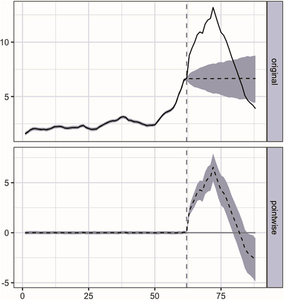
Figure 6
Professional inflation expectations in Poland. Note: During the post-intervention period, the response variable had an average value of approximately 8.98. In contrast, we would have expected an average response of 6.65 in the absence of war. The 95% interval of this counterfactual prediction is [5.35, 7.96]. The causal effect (obtained by subtracting the prediction from the response) is 2.33, with a 95% interval of [1.02, 3.63]. In relative terms, the response variable showed an increase of +36%. The 95% interval of this percentage is [+13%, +68%]. This means that the positive effect observed during the intervention period is unlikely to be due to random fluctuations.
Source: Author’s contribution.
Table 2
Results of the Chow test for a structural break at the outbreak of the war.
| Country | Expectations | Test statistic | p-Value |
|---|---|---|---|
| Ukraine | Consumers | 0.248 | 0.620 |
| Professionals | 3.039 | 0.085 | |
| Poland | Consumers | 5.272 | 0.024 |
| Professionals | 13.064 | 0.001 |
Note: The null hypothesis is that the tendencies are the same in both periods. Small p-values indicate the rejection of the hypothesis (the existence of a break). We analyse the changes in the expectations.
Source: Author’s contribution.