

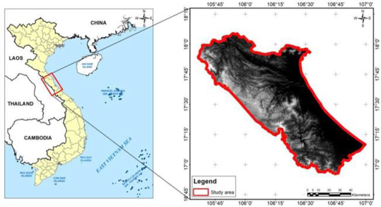
Figure 1:
Study area
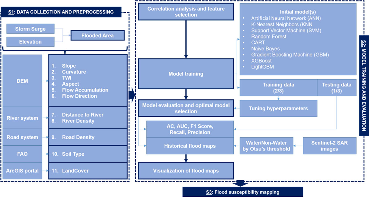
Figure 2:
Research framework
Table 1:
Mathematical foundations and roles of applied machine learning algorithms
| No. | Machine learning algorithm | Mathematical basis | Application / Reference |
|---|---|---|---|
| 1 | ANN | Multi-layer network for nonlinear pattern learning (Rumelhart et al., 1986). | |
| 2 | KNN | Instance-based learning using Minkowski distance (Cover & Hart, 1967). | |
| 3 | SVM | Maximum-margin hyperplane classifier (Cortes & Vapnik, 1995). | |
| 4 | CART | Recursive binary splitting to minimize impurity (Breiman & Ihaka, 1984). | |
| 5 | RF | Ensemble of decision trees with bootstrap aggregation (Ho, 1995; Breiman, 2001). | |
| 6 | Naive Bayes | Probabilistic classifier with conditional independence (Mitchell, 1997). | |
| 7 | GBM | Sequential additive model minimizing loss (Friedman, 2001). | |
| 8 | XGBoost | Optimized regularized boosting where Ω(ft) is optimized with histogram-based splitting to enhance efficiency on large datasets (Chen & Guestrin, 2016). | |
| 9 | LightGBM | Leaf-wise histogram-based gradient boosting where Ω(ft) is optimized with histogram-based splitting to enhance efficiency on large datasets (Ke et al., 2017). |
Table 2:
Hyperparameters and grid search of applied machine learning algorithms
| No. | Machine learning algorithms | Hyperparameters | Grid search |
|---|---|---|---|
| 1 | ANN | size, decay | size = {3, 5, 7}; decay = {0.1, 0.01, 0.001} |
| 2 | KNN | k | k = {3, 15, 2} |
| 3 | SVM | C, σ | tuneLength = 10 |
| 4 | CART | cp | tuneLength = 10 |
| 5 | RF | mtry | mtry = {2, 4, 6, 8}; ntree = 500 |
| 6 | Naive Bayes | laplace | laplace = {0, 0.5, 1, 2} |
| 7 | GBM | n.trees, depth, shrinkage, minobsinnode | n.trees = {50–300}; depth = {1, 3, 5}; shrinkage = {0.01, 0.05, 0.1}; minobsinnode = {10, 20} |
| 8 | XGBoost | nrounds, max_depth, eta, subsample, colsample_bytree, gamma | nrounds = {100, 200}; max_depth = {3, 6}; eta = {0.05, 0.1}; subsample = 0.8; colsample_bytree = 0.8 |
| 9 | LightGBM | num_leaves, learning_rate, feature_fraction, bagging_fraction, early_stopping_rounds | num_leaves = 31; learning_rate = 0.1; feature_fraction = 0.8; bagging_fraction = 0.8; early_stopping = 20 |
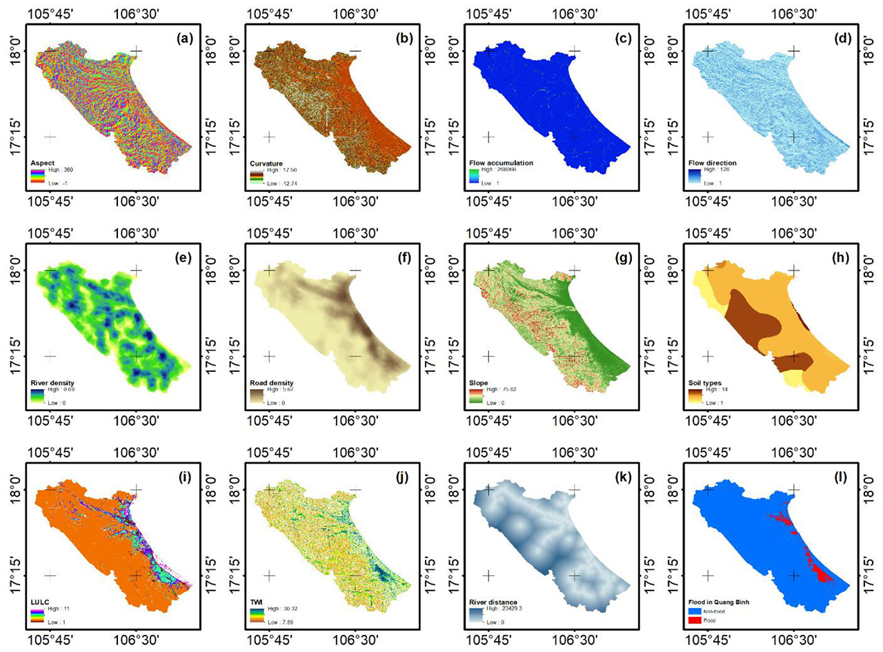
Figure 3:
Flood controlling factors: (a) Aspect, (b) Curvature, (c) Flow accumulation, (d) Flow direction, (e) River density, (f) Road density, (g) Slope, (h) Soil types, (i) LC, (j) TWI, (k) Distance to river, (l) Flood in Quang Binh based on DEM
Table 3:
Information on applied flood controlling factors
| No. | Flood controlling factors | Value (Min-Max) | Data sources and equations |
|---|---|---|---|
| 1 | Aspect | 0 – 360° | Derived from DEM (Aspect Tool/Arcmap) |
| 2 | Curvature | −12.74 – 17.50 | Derived from DEM (Curvature Tool/Arcmap) |
| 3 | Flow accumulation | 1 – 268066 | Derived from flow direction with D8 flow direction type and represented the total accumulated flow for each cell (Flow Accumulation Tool/Arcmap) |
| 4 | Flow direction | 1 – 128 | Derived from DEM, used D8 flow direction type, and values were based on neighboring flow cells (Flow Direction Tool/Arcmap) |
| 5 | River density | 0 – 0.69 | River density in a given neighbor (km/km2) (Line Density/Arcmap) |
| 6 | Road density | 0 – 5.67 | Road density in a given neighbor (km/km2) (Line Density/Arcmap) |
| 7 | Slope | 0 – 75.62° | Derived from DEM (Slope Tool/Arcmap) |
| 8 | Soil types | 1 – 14 (Representative for each soil type) | Downloaded at https://www.fao.org/soils-portal |
| 9 | LC | 1 – 11 (Representative for each type of LC) | Downloaded at https://livingatlas.arcgis.com/landcover/ |
| 10 | TWI | 7.89 – 30.32 |
α: The amount of water contained in every pixel (flow accumulation), or specific area through a certain point per unit Contour length β: Slope gradient (radians) |
| 11 | Distance to river | 0 – 23429 | Calculated, for each cell, the distance to the closest source (Euclidean Distance/Arcmap) |
Table 4:
Downloaded satellite image
| Satellite | Name | Mode | Orbit pass | Relative orbit | Time |
|---|---|---|---|---|---|
| Sentinel-1 | S1A_IW_GRDH_1SDV_20201018T11053 2_20201018T110557_034850_041018_E503 | IW | ASCENDING) | 128 | 2020-10-18 11:05:32 |
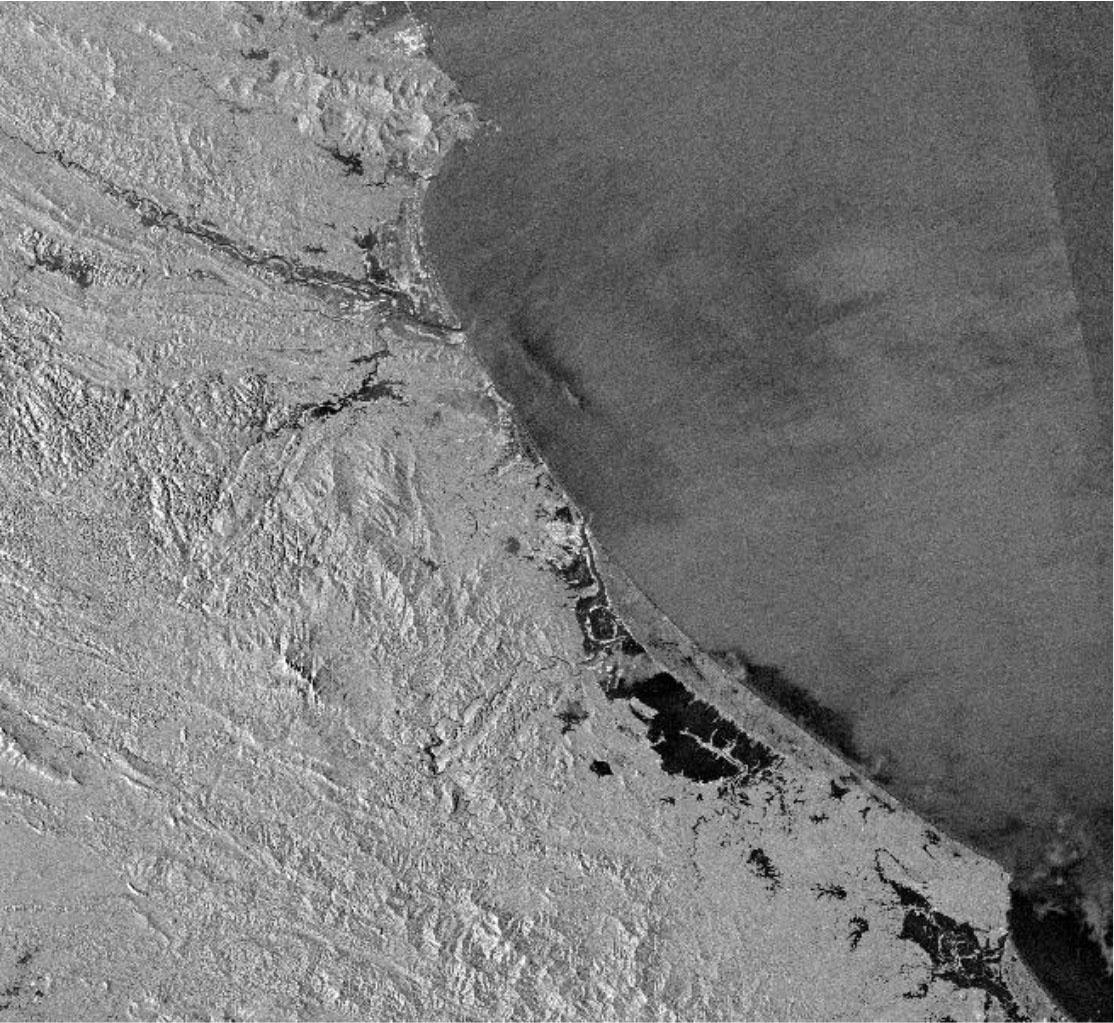
Figure 4:
Sentinel-1 satellite image in Quang Binh province (18/10/2020)
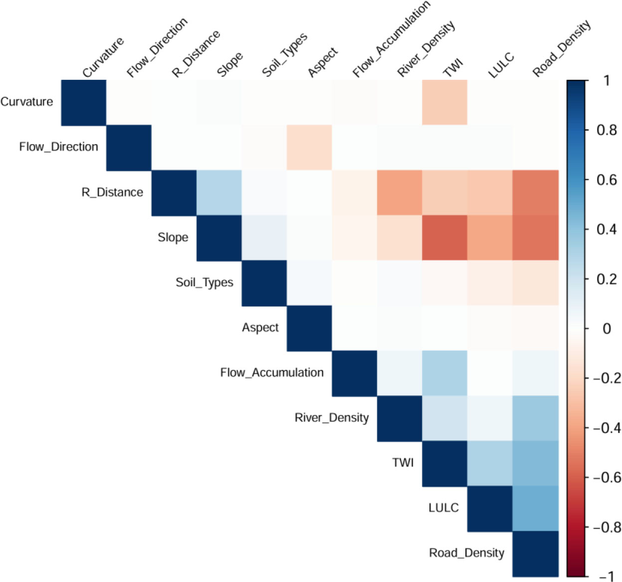
Figure 5:
Pearson correlation among applied flood controlling factors
Table 5:
Optimal hyperparameters of applied machine learning algorithms
| No. | Machine learning algorithms | Optimal hyperparameters |
|---|---|---|
| 1 | ANN | size = 3; decay = 0.1 |
| 2 | KNN | k = 15 |
| 3 | SVM | sigma = 0.0891; C = 128 |
| 4 | CART | cp = 0.00071 |
| 5 | RF | mtry = 2 |
| 6 | Naive Bayes | laplace = 0 |
| 7 | GBM | n.trees = 300; depth = 5; shrinkage = 0.05; minobsinnode = 20 |
| 8 | XGBoost | nrounds = 200; max_depth = 6; eta = 0.05; colsample_bytree = 0.8; subsample = 0.8; min_child_weight = 1 |
| 9 | LightGBM | num_leaves = 31; learning_rate = 0.1; feature_fraction = 0.8; bagging_fraction = 0.8; bagging_freq = 5 |
Table 6:
Accuracy assessment of applied machine learning algorithms
| No. | Model | Accuracy | AUC | Precision | Recall | F1 |
|---|---|---|---|---|---|---|
| 1 | ANN | 0.9716 | 0.9847 | 0.7703 | 0.3314 | 0.4634 |
| 2 | KNN | 0.9626 | 0.8205 | 0.2500 | 0.0058 | 0.0114 |
| 3 | SVM | 0.9755 | 0.9810 | 0.8021 | 0.4477 | 0.5746 |
| 4 | CART | 0.9811 | 0.9675 | 0.7763 | 0.6860 | 0.7284 |
| 5 | RF | 0.9821 | 0.9942 | 0.8678 | 0.6105 | 0.7167 |
| 6 | Naive Bayes | 0.9202 | 0.9790 | 0.3126 | 0.9651 | 0.4723 |
| 7 | GBM | 0.9834 | 0.9941 | 0.8065 | 0.7267 | 0.7645 |
| 8 | XGBoost | 0.9841 | 0.9948 | 0.8311 | 0.7151 | 0.7688 |
| 9 | LightGBM | 0.98450.9845 | 0.9942 | 0.8289 | 0.7326 | 0.7778 |
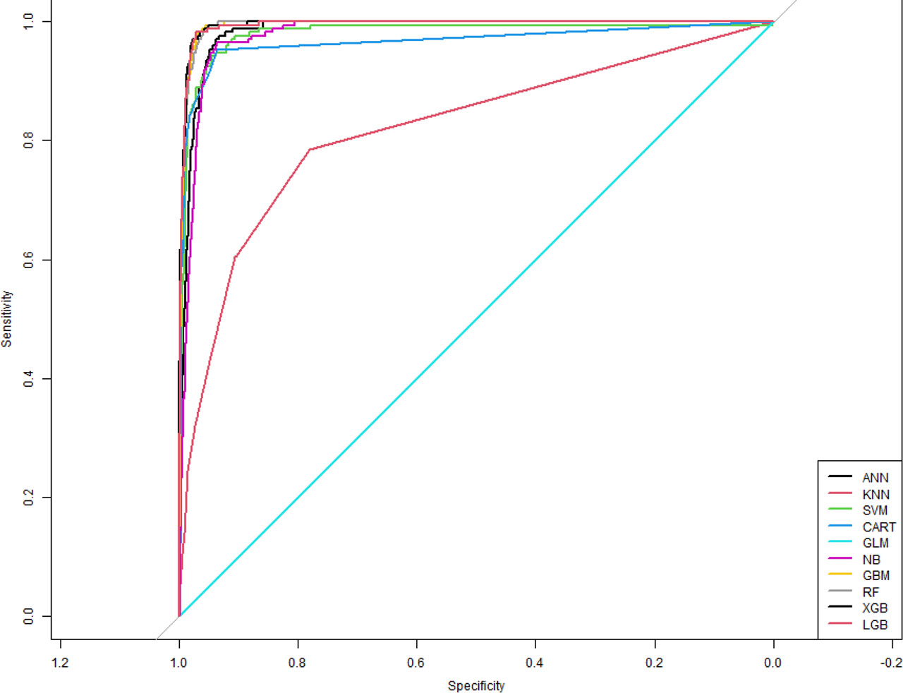
Figure 6:
ROC results of applied machine learning algorithms
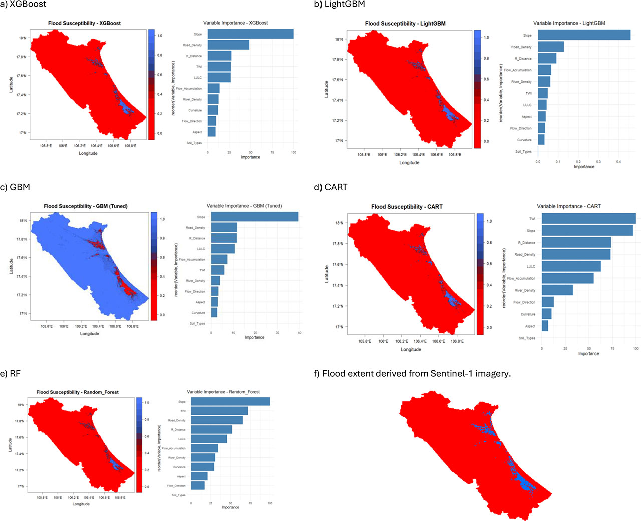
Figure 7:
Flood susceptibility mapping and relevance of factors from machine learning algorithms, and flood interpretation from satellite image