

1. Introduction
Flood risk has become an increasingly critical challenge in many coastal and riverine regions worldwide, where rapid socio-economic development coincides with growing exposure to extreme hydrometeorological events. In Vietnam, the central coastal region is particularly vulnerable to recurrent flooding due to the combined influences of complex topography, dense river networks, and frequent tropical storms (Luu et al., 2021; Seydi et al., 2022). Quang Binh province represents a typical example of this vulnerability, having experienced severe and widespread flooding during recent extreme events. In October 2020, an exceptional flood affected all districts of the province, inundating more than 1,000 residential areas, along with schools, medical facilities, and critical infrastructure (Luu et al., 2023). These impacts highlight an urgent need for reliable and spatially explicit flood susceptibility assessment approaches to support disaster prevention, risk mitigation, and long-term planning in coastal provinces of Vietnam.
Hydrological and hydraulic models (HEC-RAS, MIKE FLOOD, MIKE SHE, FVCOM, etc.), which are numerical models based on hydrological-hydraulic equations to simulate river flows and floodplains, are frequently used in traditional flood modelling techniques. For instance, groundwater and surface flow in the Argeșel River Basin were simulated using the MIKE SHE models (Sandu & Vîrsta, 2015). The MIKE FLOOD model was also applied to assess flood risk in the Mahanadi River Delta, India, under a climate change context in 2024 (Jena et al., 2024). In the same year, according to the study by Sara and her colleagues (Zahran et al., 2024), by simulating water levels and flows with the HEC-RAS model, the effects of Al-Qaraqoul Canal restoration were evaluated in Egypt. Additionally, the HEC-RAS 2D model was used to develop flood maps in the analysis of the flood impacts in the Wadi Al-Arj region of Saudi Arabia (El-Haddad et al., 2025). In a similar vein, Thanh Nguyen Thi and colleagues (2025) conducted a sensitivity analysis of the WRF-Hydro model’s parameters for simulating multi-peak flood flows in Vietnam’s Ve River basin, revealing that streamflow is highly responsive to changes in REFKDT, DKSAT, SMCMAX, and MannN under varying soil moisture conditions, while less sensitive to OVROUGHRTFAC and RETDEPRTFAC, thus optimizing the model for prolonged flood events (Nguyen et al., 2025). Doan Quang Tri and his colleagues (2026) (Tri et al., 2026) integrated the NAM–MIKE 11–LSTM modelling framework to forecast water levels in the Red River–Thai Binh River system, achieving high predictive accuracy (NSE = 0.97), thereby demonstrating the strong potential of hybrid machine learning–hydraulic approaches in Vietnam. Doan Quang Tri and his colleagues (2026) (Tri et al., 2026) integrated the NAM–MIKE 11–LSTM modelling framework to forecast water levels in the Red River–Thai Binh River system, achieving high predictive accuracy (NSE = 0.97), thereby demonstrating the strong potential of hybrid machine learning–hydraulic approaches in Vietnam. Complementing these numerical simulations, multi-criteria decision-making techniques integrated with remote sensing (RS) and GIS have proven effective for flood hazard mapping in data-scarce or complex terrains. For example, Al-Omari Tri and his colleagues (2024) (Al-Omari et al., 2024) utilized RS and GIS techniques combined with the Analytic Hierarchy Process (AHP) to develop a comprehensive flood hazard map for the vicinity of King Talal Dam in Jordan, incorporating factors such as terrain slope, elevation, aspect, proximity to water streams, drainage density, and land use/land cover to categorize flood risk levels from very low to very high, providing a robust framework for environmental management and disaster mitigation in similar arid and semi-arid regions.
These models are evident to provide a solid theoretical basis, remarkably efficient research, and management of water resources. However, construction requires detailed input data, complex configuration, and ample calculation time, so it is still limited in wide application on a large scale or in conditions of data shortage.
Flood mapping based on digital elevation models (DEMs) is a relatively straightforward approach, in which assumed flood levels are compared with terrain elevation to delineate inundated areas. This method has been widely applied at global and regional scales, including large river basins such as the Amazon and Mekong within the SHIFT (2024) project (Zheng et al., 2024), as well as in Vietnam for flood mapping and sea level rise scenario analysis (Ngoc et al., 2017; MONRE, 2012). However, previous studies have shown that flood mapping accuracy is strongly influenced by DEM type and error correction techniques, particularly in complex or urbanized terrains (Hawker et al., 2024), and that the neglect of dynamic hydrological processes (e.g., flow, discharge, and flood propagation) limits its reliability.
As a solution for the limitations, machine learning has been studied and employed in flood forecasting and simulation in numerous recent research studies. This approach can model complex relationships between natural factors and flooding based on historical data, without requiring the construction of flow equations. Thereby, machine learning models can exploit multivariate data sets (terrain, meteorology, soil, etc.) to the fullest and capture potential nonlinear relationships, helping to forecast flood areas more accurately. Many studies around the world have demonstrated the potential of ML in flood mapping.
For instance, an artificial neural network (ANN) model was compared with the HEC-RAS hydraulic model for flood forecasting, and the ANN model achieved a correlation coefficient exceeding 0.90 due to its ability to capture real-time flood dynamics (Agudelo-Otálora et al., 2018). Moreover, based on hydrological, topographic, and urban data, Qin et al. (2025) employed random forest (RF) to estimate urban flood mapping for the Guangzhou region (China), producing reasonably accurate findings. Jun Liu et al. (2021) achieved an excellent accuracy (model AUC > 0.9) in mapping the flood susceptibility of the region using a Support Vector Machine (SVM) and 11 geographical variables. The SVM successfully identified flood areas (Southeast Asia and South Asia), comprising a considerable fraction of high-risk areas. Additionally, Panahi et al.’s (2025) work employed eight layers of geo-environmental data and 6682 historical flood occurrences from throughout the world to train the SVR model (parameter optimization using GWO/WOA), resulting in a global flood susceptibility map. The results highlighted the most flood-prone areas in Southeast Asia, South Asia, West Africa, and Southeast America; notably, the top 5 countries in terms of flood-prone area ratio were the United States, Indonesia, India, Brazil, and Nigeria. In Vietnam, Chinh Luu et al. (2021) integrated the Partial Decision Tree (PART) algorithm with ensemble techniques (AdaBoost, Bagging, Dagging, Random Subspace) to flood mapping in Quang Binh province. The findings confirmed the great potential of machine learning methods (AUC > 0.9) in simulating floods in the study area.
In the context of this study, the aim was to develop an approach for mapping accurate and appropriate flood susceptibility in Vietnam using efficient machine learning algorithms and multiple topographic and hydrological variables. The flood event in Quang Binh around 11:00 a.m. on October 18, 2020, when the sea level increased to 1.84 m and rainfall was not the primary cause, was selected as a typical case. Contrasting with most previous work, which employed rainfall as the primary input variable, this one focused on mapping flood susceptibility in relation to tides and storm surges (or storm-induced water level rise). While effectively representing the unique flooding process of the Central Vietnamese coastal region, excluding rainfall helps highlight the impact of hydrological parameters in the model. This implies the ability to simulate flood scenarios in response to fluctuating hydrological and meteorological variables, in addition to enabling flexible modelling of flood susceptibility mapping at any given time. Nine modern machine learning algorithm models (ANN, KNN, SVM, CART, Naive Bayes, GBM, RF, XGBoost, and LightGBM) were applied and evaluated. In addition, the models were trained on not only a dataset of storm-induced water level rise and historical flood, but also a set of 11 topographic and hydrological variables (Slope, Aspect, Curvature, Flow direction, Flow accumulation, Topographic wetness index, Land cover, Soil type, River density, Road density, and Distance to river) to improve the efficiency and accuracy. This study was expected to significantly enhance the quality of flood susceptibility maps in the context of sea level rise in Vietnam, thereby identifying areas prone to high potential flooding, preventing and minimizing flooding damage, and providing more effective support for planning and disaster prevention.
2. Methodology
2.1. Description of Study Area
Quang Binh Province, located in the North Central Coast region of Vietnam, covers an area of approximately 8,065 km2, with diverse terrain ranging from mountainous areas in the West to low-lying coastal plains in the East. It is affected by a tropical monsoon climate, with high rainfall, especially from September to November, causing flash floods and inundation. In addition, major river systems such as the Nhat Le River and Gianh River also increase the risk of flooding. According to previous studies (Luu et al., 2021; Ha et al., 2023), approximately 10.4% (829 km2) and 3.36% (27,121 ha) of the province have experienced very high and extreme risk of flooding, respectively, in the rainy season.
The 2020 historical flood in Quang Binh, one of the most severe extreme weather events on record, occurred in October 2020 due to the consecutive impacts of significant storms, including Linfa, Nangka, Saudel, and Molave, causing heavy rain and tornadoes in the central provinces of Vietnam (Luu et al., 2023). On major rivers, water levels were recorded to exceed those of previous historical floods (1950, 1979, 1999, 2007, 2010, and 2016). In particular, 1,014 residential areas, 70 schools, 13 health facilities, 32,558 ha of agricultural areas, 402 km of roads, 29 km of railways, 35 road bridges, and 239 businesses were inundated in the floodplain (Luu et al., 2023). These impacts underscore the need for spatial analysis techniques to map flood impacts, a crucial step in supporting risk management and post-disaster recovery.
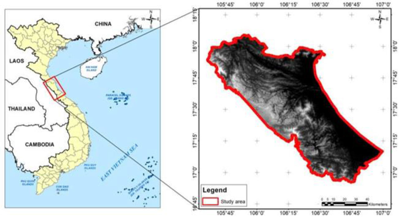
Figure 1:
Study area
2.2. Methods
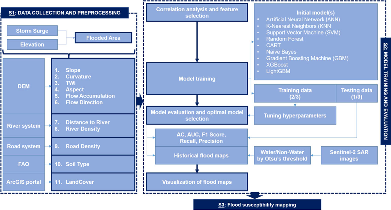
Figure 2:
Research framework
The study was structured into three main steps: data collection and preprocessing, model training and evaluation, and flood susceptibility mapping (Figure 2). Storm-induced water level data from the Dong Hoi hydrological station and Sentinel-1 imagery were used to generate flood labels based on a 10 m digital elevation model (DEM). A total of 11 geo-environmental variables were prepared, including six DEM-derived topographic factors (aspect, curvature, flow accumulation, flow direction, slope, and topographic wetness index) and five ancillary variables (river density, road density, soil type, land cover, and distance to river), all standardized to a 10 m spatial resolution. Pearson correlation analysis was applied for variable selection. Nine machine learning algorithms (ANN, KNN, SVM, CART, Naive Bayes, GBM, RF, XGBoost, and LightGBM) were trained using a 70:30 training–testing split with hyperparameter optimization via grid search and five-fold cross-validation. Model performance was evaluated using Accuracy, AUC, Recall, Precision, and F1, and the best-performing models were used to generate and validate flood susceptibility maps based on Sentinel-1–derived flood extents.
2.2.1. Flood Controlling Factors
A set of eleven topographic and hydrological factors was chosen to develop a flood susceptibility map based on a comprehensive and careful analysis of previous studies on flood susceptibility (Agassi et al., 1990; Wang et al., 2015; Costache & Zaharia, 2017; Shafizadeh-Moghadam et al., 2018; El-Haddad et al., 2021; Bui et al., 2021; Nguyen et al., 2023) and the specific characteristics of the study area (Luu et al., 2021).
2.2.1.1. Aspect
Aspect is an important topographic variable in flood susceptibility assessment. Various studies have shown that aspect determines the “path” of runoff — places with an aspect facing low-lying areas, away from the sea/river, tend to hold more water, because the runoff cannot drain as quickly, leading to a higher risk of flooding (Agassi et al., 1990).
2.2.1.2. Curvature
Curvature explicating the shape of the terrain surface has a significant influence on surface runoff and water accumulation capacity. While positive values (convex) indicate high terrain supporting the dispersal of water easily, negative values (concave) associated with low-lying areas tend to accumulate water and increase the risk of flooding (Zevenbergen & Thorne, 1987).
2.2.1.3. Flow Accumulation
Flow accumulation is used as a topographic input variable reflecting the ability to concentrate flow on the surface. Areas with high accumulation values are often places where water from upstream is concentrated, receiving flows from many other places, increasing the risk of local flooding. This is one of the key indicators that helps the model identify areas prone to flooding under high water conditions (Tehrany et al., 2014).
2.2.1.4. Flow Direction
Flow direction is the direction in which water flows over the terrain surface, usually calculated from a DEM using algorithms such as D8. This index indicates which cell the water from each raster will flow to next, identifying the main water flow, water accumulation areas, and flow bottlenecks. Areas located downstream of the main flow direction or near the accumulation area tend to be more prone to flooding due to limited drainage capacity (Kaya & Derin, 2023).
2.2.1.5. River Density
River density reflects the level of development of the natural drainage system in a specific area. High river density values usually indicate better drainage capacity; however, in some cases, if the system is overloaded or congested, flooding may occur easily (Jahanbani et al., 2024).
2.2.1.6. Road Density
Like river density, road density represents the density of roads in a specific area. High road density can increase the risk of flooding by increasing impervious surface area and reducing the efficiency of surface water drainage (Jahanbani et al., 2024).
2.2.1.7. Slope
Slope or steep slope increases surface runoff velocity and reduces soil infiltration, while a low slope increases the likelihood of flooding (Agassi et al., 1990).
2.2.1.8. Soil Type
Soil type is another parameter commonly used in flood susceptibility mapping. The soil type of a catchment controls the amount of water that infiltrates into the soil and thus the volume of rainfall that will cause flooding (indirectly, the rate of development and intensity of the flood) (Kaya & Derin, 2023).
2.2.1.9. Land Cover
Land cover is an important factor in flood assessment due to its direct impact on water infiltration capacity, surface runoff velocity, and natural water retention (Kaya & Derin, 2023).
2.2.1.10. Topographic Wetness Index (TWI)
The topographic wetness index (TWI) is a spatial hydrological variable that reflects the tendency of the terrain to store water, calculated from the flow accumulated and slope. High TWI values indicate areas that are prone to water storage due to flat terrain and receiving runoff from large upstream areas, thereby increasing the risk of flooding (Kaya & Derin, 2023).
2.2.1.11. Distance to River
Distance to river is an important factor in flood analysis, especially in areas along rivers or downstream of coastal rivers. Areas located near rivers are often more susceptible to flooding due to direct impact from flood flows, storm surges, or high tides (Tehrany et al., 2019).
2.2.2. Machine Learning Algorithms
In this study context, nine machine learning algorithms (ANN, KNN, SVM, CART, Naïve Bayes, GBM, RF, XGBoost, and LightGBM) were chosen for use to ensure principal flexibility and the capacity to simulate the nonlinear relationship between input parameters and floods. The combination of multiple algorithms allows for comparing the performance and selecting the optimal model for flood susceptibility mapping. In particular, the boosting group (GBM, XGBoost, LightGBM), a new generation group, is favoured due to its superior performance and ability to handle large, noisy, and unbalanced data well. Despite not being the latest algorithms, they are currently the industry standard for group data analysis and are frequently applied to GIS, environmental, and natural catastrophe issues (Friedman, 2001; Chen & Guestrin, 2016; Ke et al., 2017).
2.2.2.1. Artificial Neural Network (ANN)
An artificial neural network (ANN) (Goodfellow et al., 2016) is a mathematical model designed based on the simulation of the structure and operation of biological neural networks in the human brain, including many processing nodes called artificial neurons, organized into consecutive interacting layers (input layer, hidden layers, output layer). Each neuron receives input information through connections, then calculates based on a nonlinear activation function to generate an output signal.
2.2.2.2. K-Nearest Neighbours (KNN)
The K-Nearest Neighbours (KNN) algorithm is a non-parametric machine learning method, based on the theory of similarity between observations, commonly used in classification and regression problems (Cover & Hart, 1967). The main idea of the algorithm is to determine the k data points that are closest (based on some distance measure such as Euclidean, Manhattan, or Minkowski) to the new data point to be predicted, and then use the most frequent result (classification) or the average value (regression) of these neighbour points as the prediction for the new point (Altman, 1992).
2.2.2.3. Support Vector Machine (SVM)
Support Vector Machine (SVM) (Cortes & Vapnik, 1995) is a supervised machine learning algorithm built on the principle of maximizing the margin between data classes, first introduced by Vapnik and colleagues. In the mechanism of SVM, an optimal hyperplane is constructed in the feature space to separate data classes most clearly. The data points closest to the separating hyperplane are called support vectors, which play a decisive role in determining the decision margin of the model.
2.2.2.4. Classification and Regression Trees (CART)
Classification and Regression Trees (CART) are a supervised machine learning algorithm proposed by Breiman et al. (2017) to solve classification and regression problems through decision tree structures. The main idea of CART is to build a binary tree by continuously dividing the data set based on input variables, aiming to optimize a specific criterion such as purity (gini impurity or entropy) in classification problems or the sum of squared errors in regression problems (Hastie et al., 2009).
2.2.2.5. Random Forest (RF)
Random Forest (RF) algorithm, introduced by Breiman (2001), is a supervised machine learning technique based on the idea of ensemble learning, in which multiple independent decision trees are trained on random subsets of data, using bootstrap sampling and random feature selection. The final prediction of the RF model is made through the principle of majority voting in the classification problem or taking the average value in the regression problem from all the component trees (Liaw & Wiener, 2002).
2.2.2.6. Naive Bayes
The Naive Bayes algorithm is a supervised machine learning method based on Bayes’ theorem, built on the simplifying assumption that all features (input variables) are conditionally independent of each other when considered in each data class (Mitchell, 1997). Although this assumption is not valid in most practical cases, it helps the algorithm significantly simplify probability calculations, thereby making this algorithm highly scalable and computationally efficient (Russell & Norvig, 2016).
2.2.2.7. Gradient Boosting Machine (GBM)
Gradient Boosting Machine (GBM) (Friedman, 2001) is a supervised machine learning algorithm based on boosting, an ensemble learning method that sequentially combines multiple weak learners, usually decision stumps or shallow trees, to form a stronger model with superior predictive ability. GBM works by constructing each new decision tree to minimize the loss function through gradient descent, focusing on overcoming residual errors from the previous model.
2.2.2.8. Extreme Gradient Boosting (XGBoost)
Extreme Gradient Boosting (XGBoost) is a machine learning algorithm based on the gradient tree boosting model, developed by Chen and Guestrin (2016). This algorithm improves the classical Gradient Boosting Machine (GBM) technique by integrating efficient optimization solutions, especially in building decision trees and optimizing loss functions.
2.2.2.9. Light Gradient Boosting Machine (LightGBM)
Light Gradient Boosting Machine (LightGBM) (Ke et al., 2017) is a gradient boosting machine learning algorithm developed by Microsoft Research with the goal of increasing computational efficiency and scalability for large datasets. This algorithm improves on traditional gradient boosting models such as GBM and XGBoost by applying leaf-wise growth instead of level-wise growth. This helps LightGBM significantly reduce the depth of the tree, speed up data processing, and improve prediction accuracy.
Table 1:
Mathematical foundations and roles of applied machine learning algorithms
| No. | Machine learning algorithm | Mathematical basis | Application / Reference |
|---|---|---|---|
| 1 | ANN | Multi-layer network for nonlinear pattern learning (Rumelhart et al., 1986). | |
| 2 | KNN | Instance-based learning using Minkowski distance (Cover & Hart, 1967). | |
| 3 | SVM | Maximum-margin hyperplane classifier (Cortes & Vapnik, 1995). | |
| 4 | CART | Recursive binary splitting to minimize impurity (Breiman & Ihaka, 1984). | |
| 5 | RF | Ensemble of decision trees with bootstrap aggregation (Ho, 1995; Breiman, 2001). | |
| 6 | Naive Bayes | Probabilistic classifier with conditional independence (Mitchell, 1997). | |
| 7 | GBM | Sequential additive model minimizing loss (Friedman, 2001). | |
| 8 | XGBoost | Optimized regularized boosting where Ω(ft) is optimized with histogram-based splitting to enhance efficiency on large datasets (Chen & Guestrin, 2016). | |
| 9 | LightGBM | Leaf-wise histogram-based gradient boosting where Ω(ft) is optimized with histogram-based splitting to enhance efficiency on large datasets (Ke et al., 2017). |
2.2.2.10. Tuning Hyperparameters
To select the optimal hyperparameters for each machine learning model, a combination of two techniques (5-fold cross-validation and grid search) was employed. In particular, cross-validation is a technique for evaluating model performance that aims to reduce bias caused by random data splitting. In k-fold cross-validation (Breiman et al., 2017), the training set is divided into k equal parts; the model is trained on k-1 parts and tested on the remaining parts. The process is repeated k times, each time retaining a different part for evaluation. The average of the results of k rounds of validation is used as the model performance index. Besides, grid search is a method for systematically searching the hyperparameter space. A grid of possible values is predefined for each hyperparameter, and all combinations in this grid are tested through cross-validation. The combination that gives the best result (e.g., highest AUC) is selected to train the final model (Bergstra & Bengio, 2012). Combining these two methods supports to ensure systematic selection of optimal hyperparameters, while increasing the stability and generalizability of the model.
Table 2:
Hyperparameters and grid search of applied machine learning algorithms
| No. | Machine learning algorithms | Hyperparameters | Grid search |
|---|---|---|---|
| 1 | ANN | size, decay | size = {3, 5, 7}; decay = {0.1, 0.01, 0.001} |
| 2 | KNN | k | k = {3, 15, 2} |
| 3 | SVM | C, σ | tuneLength = 10 |
| 4 | CART | cp | tuneLength = 10 |
| 5 | RF | mtry | mtry = {2, 4, 6, 8}; ntree = 500 |
| 6 | Naive Bayes | laplace | laplace = {0, 0.5, 1, 2} |
| 7 | GBM | n.trees, depth, shrinkage, minobsinnode | n.trees = {50–300}; depth = {1, 3, 5}; shrinkage = {0.01, 0.05, 0.1}; minobsinnode = {10, 20} |
| 8 | XGBoost | nrounds, max_depth, eta, subsample, colsample_bytree, gamma | nrounds = {100, 200}; max_depth = {3, 6}; eta = {0.05, 0.1}; subsample = 0.8; colsample_bytree = 0.8 |
| 9 | LightGBM | num_leaves, learning_rate, feature_fraction, bagging_fraction, early_stopping_rounds | num_leaves = 31; learning_rate = 0.1; feature_fraction = 0.8; bagging_fraction = 0.8; early_stopping = 20 |
2.2.2.11. Accuracy Assessment
In machine learning, the model evaluation of the classification performance was implemented with various metrics, such as Accuracy, AUC, Precision, Recall, F1, Specificity, Matthews Correlation Coefficient (MCC), Cohen’s Kappa, etc. However, in the study framework, five metrics (AC (1), AUC, Recall (2), Precision (3), and F1 (4)) were selected to ensure the simultaneous evaluation of the overall performance and the ability to distinguish between two data classes (flooded and non-flooded). In particular:
Accuracy (AC): The proportion of observations that are correctly classified across the entire test set. This metric reflects overall accuracy but can be skewed when the data is imbalanced (Huang & Huang, 2023).
Area Under the Curve (AUC): The area under the Receiver Operating Characteristic (ROC) curve represents the ability to discriminate between two classes over the entire threshold range. An AUC close to 1 indicates a good classification model, while an AUC = 0.5 is equivalent to random classification (Ling et al., 2003).
Recall (Sensitivity): The proportion of observations in the positive class (flooded). High recall reflects that the model rarely misses flooded areas (Hicks et al., 2022).
Precision: The percentage of correct flood predictions. High precision reflects the model’s reliability in issuing flood warnings (Davis & Goadrich, 2006).
F1: The average of Precision and Recall, used to evaluate the balance between detection ability (Recall) and prediction accuracy (Precision). F1 is beneficial when the data is imbalanced (Vakili et al., 2020).
2.3. Data Sources
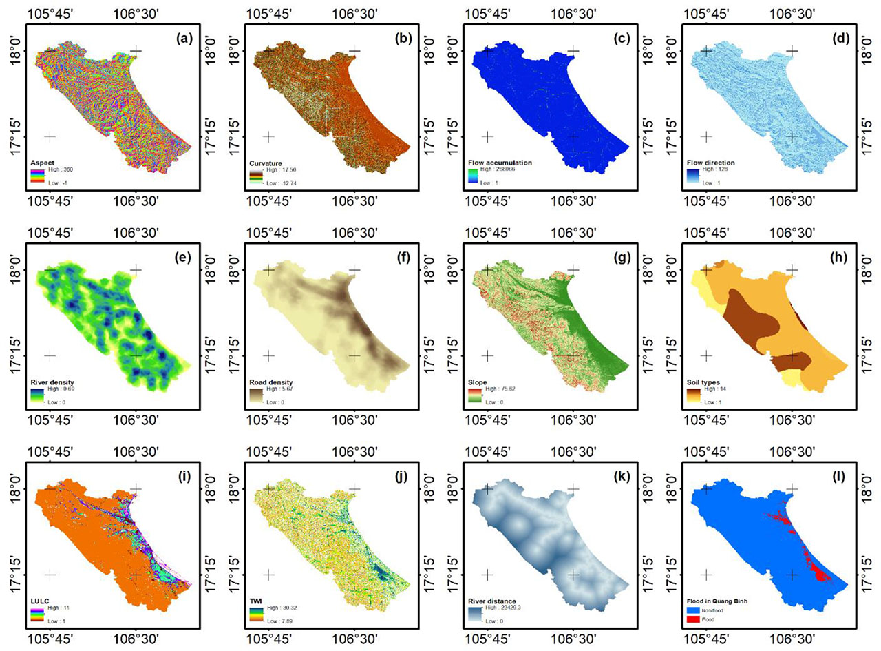
Figure 3:
Flood controlling factors: (a) Aspect, (b) Curvature, (c) Flow accumulation, (d) Flow direction, (e) River density, (f) Road density, (g) Slope, (h) Soil types, (i) LC, (j) TWI, (k) Distance to river, (l) Flood in Quang Binh based on DEM
Based on the selected topographic and hydrological factors for flood susceptibility mapping, the key data sources were collected, including: land cover with 10 m resolution extracted from Esri platform; soil data collected from the global database of the Food and Agriculture Organization of the United Nations (FAO); and digital elevation model (DEM) at a scale of 1:10,000 provided by the Department of Surveying, Mapping and Geographic Information of Vietnam. DEM was used to derive topographic indices such as aspect, curvature, slope, TWI, flow direction, and flow accumulation. River and transportation network data were obtained from a 1:25,000 scale geodatabase, serving to analyse factors such as river density, distance to river, and road density. (Figure 3 and Table 3).
Table 3:
Information on applied flood controlling factors
| No. | Flood controlling factors | Value (Min-Max) | Data sources and equations |
|---|---|---|---|
| 1 | Aspect | 0 – 360° | Derived from DEM (Aspect Tool/Arcmap) |
| 2 | Curvature | −12.74 – 17.50 | Derived from DEM (Curvature Tool/Arcmap) |
| 3 | Flow accumulation | 1 – 268066 | Derived from flow direction with D8 flow direction type and represented the total accumulated flow for each cell (Flow Accumulation Tool/Arcmap) |
| 4 | Flow direction | 1 – 128 | Derived from DEM, used D8 flow direction type, and values were based on neighboring flow cells (Flow Direction Tool/Arcmap) |
| 5 | River density | 0 – 0.69 | River density in a given neighbor (km/km2) (Line Density/Arcmap) |
| 6 | Road density | 0 – 5.67 | Road density in a given neighbor (km/km2) (Line Density/Arcmap) |
| 7 | Slope | 0 – 75.62° | Derived from DEM (Slope Tool/Arcmap) |
| 8 | Soil types | 1 – 14 (Representative for each soil type) | Downloaded at https://www.fao.org/soils-portal |
| 9 | LC | 1 – 11 (Representative for each type of LC) | Downloaded at https://livingatlas.arcgis.com/landcover/ |
| 10 | TWI | 7.89 – 30.32 |
α: The amount of water contained in every pixel (flow accumulation), or specific area through a certain point per unit Contour length β: Slope gradient (radians) |
| 11 | Distance to river | 0 – 23429 | Calculated, for each cell, the distance to the closest source (Euclidean Distance/Arcmap) |
Besides, radar Sentinel-1 images, which were acquired at 11:00 on October 18, 2020, coinciding with the time of the historical flood in Quang Binh, were also collected to assess the spatial accuracy between the actual flood areas and the mapped flood susceptibility areas (Table 4 and Figure 4). Along with that, the water level at Dong Hoi station (reaching 1.84 m) was recorded to serve the construction of the hypothetical flood map.
Table 4:
Downloaded satellite image
| Satellite | Name | Mode | Orbit pass | Relative orbit | Time |
|---|---|---|---|---|---|
| Sentinel-1 | S1A_IW_GRDH_1SDV_20201018T11053 2_20201018T110557_034850_041018_E503 | IW | ASCENDING) | 128 | 2020-10-18 11:05:32 |
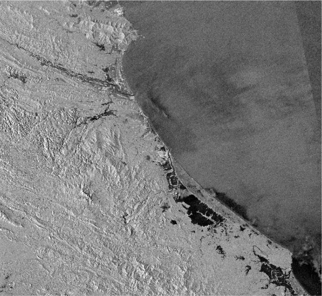
Figure 4:
Sentinel-1 satellite image in Quang Binh province (18/10/2020)
3. Results
3.1. Pearson Correlation and Tuning Hyperparameters
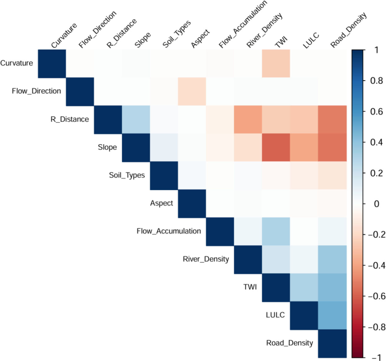
Figure 5:
Pearson correlation among applied flood controlling factors
Correlation analysis is an important step to ensure that the model is not affected by multicollinearity, which can distort the coefficients and reduce the stability of linear algorithms such as logistic regression or linear SVM. If the correlation matrix results in a pair of strongly correlated variables, one of the variables needs to be eliminated. The eliminated variable is considered based on the influence level on the dependent variable (Salih, 2024). In this study, Pearson correlation was performed to assess the linear relationship between the 11 independent variables before training the machine learning models. The results in the correlation matrix (Figure 5) demonstrated that the majority of pairs of variables had low to moderate correlation coefficients (|r| < 0.7), indicating that the risk of multicollinearity was negligible. All independent variables were used for training the nine machine learning models.
Regarding tuning hyperparameters, the hyperparameters of the nine models were fine-tuned using a 5-fold cross-validation and grid search approach to maximize the AUC. The results indicated that each model had its optimal parameters, which were summarized in Table 5. Specially, ANN, SVM, and boosting models were tuned using several parameters at the same time, such as GBM (n.trees = 300; depth = 5; shrinkage = 0.05; minobsinnode = 20), XGBoost (nrounds = 200; max_depth = 6; eta = 0.05; colsample_bytree = 0.8; subsample = 0.8; min_child_weight = 1), and LightGBM (num_leaves = 31; learning_rate = 0.1; feature_fraction = 0.8; bagging_fraction = 0.8; bagging_freq = 5).
Table 5:
Optimal hyperparameters of applied machine learning algorithms
| No. | Machine learning algorithms | Optimal hyperparameters |
|---|---|---|
| 1 | ANN | size = 3; decay = 0.1 |
| 2 | KNN | k = 15 |
| 3 | SVM | sigma = 0.0891; C = 128 |
| 4 | CART | cp = 0.00071 |
| 5 | RF | mtry = 2 |
| 6 | Naive Bayes | laplace = 0 |
| 7 | GBM | n.trees = 300; depth = 5; shrinkage = 0.05; minobsinnode = 20 |
| 8 | XGBoost | nrounds = 200; max_depth = 6; eta = 0.05; colsample_bytree = 0.8; subsample = 0.8; min_child_weight = 1 |
| 9 | LightGBM | num_leaves = 31; learning_rate = 0.1; feature_fraction = 0.8; bagging_fraction = 0.8; bagging_freq = 5 |
3.2. Accuracy Assessment of Machine Learning Models
The performance of the nine machine learning models was compared and assessed through accuracy, AUC, precision, recall, and F1 metrics on the testing data (Table 6 and Figure 6). It was shown that the Boosting group, RF, and CART algorithms outperformed the other models in classifying and detecting flooded areas. LightGBM was the best model with accuracy = 0.9845, AUC = 0.9942, and F1 = 0.7778. This also indicated a good balance between correct detection (recall = 0.733) and prediction accuracy (precision = 0.829). Similarly, XGBoost and GBM achieved high accuracy with F1 of 0.7688 and 0.7645, respectively. Besides, RF and CART demonstrated more stable performance, with accuracy exceeding 0.98 and F1 surpassing 0.71. However, the recall of RF (0.6105) and CART (0.6860) was lower than that of the Boosting group.
On the other hand, the remaining models exhibited significant variations in their accuracy metrics. SVM gained high accuracy (0.9755) and AUC (0.9810), but its F1 was only 0.5746 due to a relatively low recall (0.448). In addition, although ANN saw a very high AUC (0.9847), it experienced a low F1 (0.4634) due to poor recall (0.3314). Naive Bayes had the highest recall (0.9651) but low precision (0.313), resulting in a low F1 (0.4723). This highlighted the imbalance in the classification ability of these models. Specifically, KNN was the weakest model, with an F1 of only 0.0114 and a recall almost equal to 0 (0.006), indicating that the model failed to learn the features of the flooded layer.
Table 6:
Accuracy assessment of applied machine learning algorithms
| No. | Model | Accuracy | AUC | Precision | Recall | F1 |
|---|---|---|---|---|---|---|
| 1 | ANN | 0.9716 | 0.9847 | 0.7703 | 0.3314 | 0.4634 |
| 2 | KNN | 0.9626 | 0.8205 | 0.2500 | 0.0058 | 0.0114 |
| 3 | SVM | 0.9755 | 0.9810 | 0.8021 | 0.4477 | 0.5746 |
| 4 | CART | 0.9811 | 0.9675 | 0.7763 | 0.6860 | 0.7284 |
| 5 | RF | 0.9821 | 0.9942 | 0.8678 | 0.6105 | 0.7167 |
| 6 | Naive Bayes | 0.9202 | 0.9790 | 0.3126 | 0.9651 | 0.4723 |
| 7 | GBM | 0.9834 | 0.9941 | 0.8065 | 0.7267 | 0.7645 |
| 8 | XGBoost | 0.9841 | 0.9948 | 0.8311 | 0.7151 | 0.7688 |
| 9 | LightGBM | 0.98450.9845 | 0.9942 | 0.8289 | 0.7326 | 0.7778 |
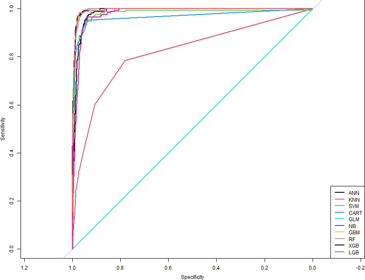
Figure 6:
ROC results of applied machine learning algorithms
3.3. Flood Susceptibility Mapping
For the five best-performing machine learning models (RF, XGBoost, LightGBM, GBM, and CART), flood susceptibility maps for the study area were constructed, in which each pixel was labelled with a flood probability value of 0 or 1. Based on this value, the index was classified into two levels: non-flood (0 – 0.6), flooded (0.6 – 1). The map was illustrated in Figure 7.
In terms of quantitative assessment, the study performed a spatial comparison between the flood susceptibility map generated by machine learning models and the real-time flood map extracted from Sentinel-1 images (Figure 7f). The real-time flood class was classified using Otsu’s method at the time of high-water levels, reflecting the flood status resulting from the combination of high tides and sea level rise.
The findings indicated that the four models (CART, RF, XGBoost, and LightGBM) exhibited high spatial correlation with the interpreted real-time flood map, with most of the simulated flooded areas matching the areas in real time, such as low-lying riverbanks, agricultural land along the dike, and low-lying residential areas. Meanwhile, GBM despite its high quantitative performance, produced inconsistent spatial distributions, with many upland areas incorrectly predicted as flooded. This highlighted the importance of visual and field assessment in model validation.
Combined with the chart of relevance of factors, four variables (slope, road density, distance to river, and TWI) were the main determinants in all five models. Specifically, the GBM and LightGBM models indicated that slope had the most considerable influence (>35%). CART and RF emphasized the role of TWI and distance to river. XGBoost demonstrated a harmonious combination of slope, road density, and TWI.
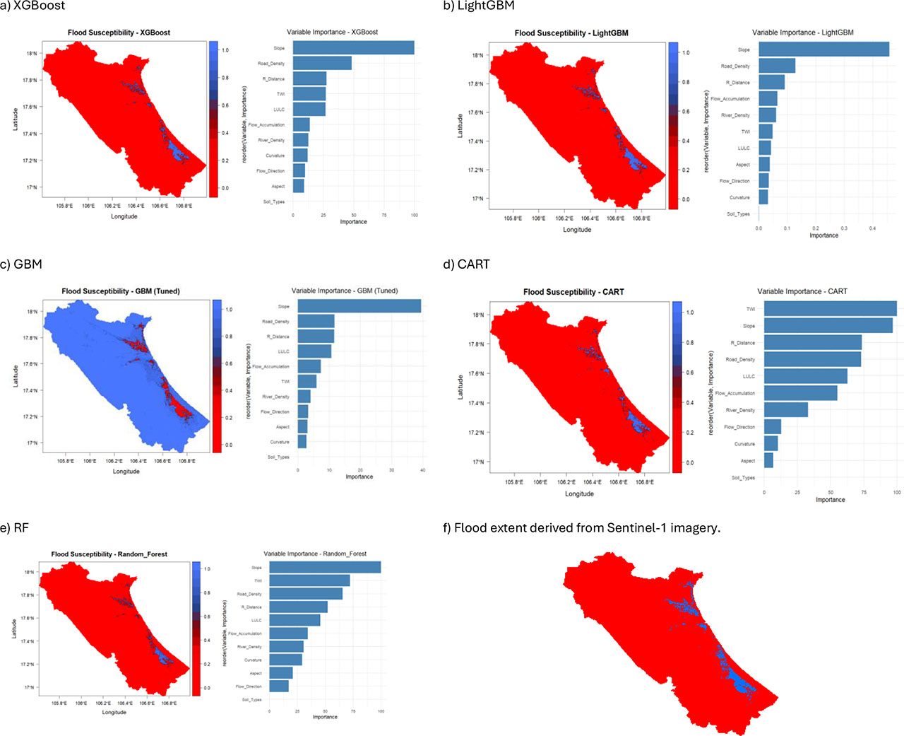
Figure 7:
Flood susceptibility mapping and relevance of factors from machine learning algorithms, and flood interpretation from satellite image
4. Discussion
4.1. Significant Flood Controlling Factors of the Study Area
The correlation and influence analysis of the factors in this study clarified the significant roles of four specific factors (slope, TWI, distance to river, and road density) in determining the possibility of flooding in Quang Binh. Specifically, slope emerged as the most influential factor (>35% in GBM and LightGBM), reflecting the direct relationship between slope and surface flow velocity, as well as the risk of flash floods in the upstream area. This finding was entirely consistent with previous studies (El-Haddad et al., 2021; Janizadeh et al., 2019), which confirmed that a steep slope increased the ability to concentrate and drain water quickly, leading to a higher risk of flooding. Furthermore, TWI was significant in pinpointing regions that were vulnerable to water accumulation, particularly in coastal plains with flat terrain and poor drainage capacity. This outcome was in line with research on flood risk assessment in the Middle East and Southeast Asia (Tehrany et al., 2014; Costache & Zaharia, 2017).
Besides, the influence of the distance to the river was also apparent. According to (Tehrany et al., 2019), regions adjacent to the Gianh and Nhat Le river systems were directly impacted by storms and river surges, rendering them more vulnerable to flooding. Road density, which reflects the function of transportation infrastructure in altering drainage surfaces and expanding impervious surface areas, was also found to be an influential contributor to exacerbating urban floods (Jahanbani et al., 2024). As a result, the combination of four flood controlling factors indicated an apparent association with the natural and economic conditions of Quang Binh province, thereby strengthening the model’s rationality when compared with published scientific evidence.
4.2. Effective Machine Learning Models for the Study Area
This study applied and compared the performance of the nine state-of-the-art machine learning models in constructing flood susceptibility maps under the influence of storm-induced water levels for Quang Binh province during the historical flood in October 2020. The findings indicated that CART, RF, XGBoost, and LightGBM achieved the highest performance in both quantitative accuracy (Accuracy > 98%, AUC > 0.99, F1 > 0.7) and spatial plausibility, with good correlation between simulated flood maps and real-time flood maps derived from Sentinel-1 imagery. The superior performance of CART, RF, XGBoost, and LightGBM was highlighted by the algorithmic advantages in handling non-linear and complex relationships between flood controlling factors. In particular, CART’s straightforward and understandable decision tree structure revealed that it could effectively capture topography and hydrological thresholds, making it especially appropriate for a variety of topographic contexts, including Quang Binh (Breiman et al., 2017). RF further improved stability and accuracy by combining multiple decision trees through bootstrap sampling techniques, thereby reducing overfitting and improving generalization over areas with significant variations in terrain and land cover (Breiman, 2001; Liu et al., 2021; Liaw & Wiener, 2002). Meanwhile, two sophisticated boosting algorithms, XGBoost and LightGBM, proved it possible to handle massive, imbalanced datasets effectively and to detect minor changes in variables (Chen & Guestrin, 2016; Ke et al., 2017). Specifically, LightGBM achieved the ideal balance of recall and precision owing to its leaf-wise tree growth technique and fast computing speed, which rendered it appropriate for simulating flood patterns in Quang Binh’s upstream mountainous regions as well as coastal plains.
Additionally, the hydrological and physical features of the study area were also associated with this adaptability. The hydrological and physical features of the province were also associated with this adaptability. Quang Binh explicitly differentiates between the high mountainous region in the west, where flash floods are likely to strike, and the low-lying coastal plain area, which is linked to a large concentration of residential areas and agricultural land (Luu et al., 2021). This feature allows CART to precisely determine the thresholds of topographic and hydrological variables (e.g., slope, TWI, and distance to river) that were directly associated with the probability of flooding. RF proved to be effective in handling heterogeneous data, simultaneously reflecting the impact of multiple environmental variables and limiting overfitting in the context of substantial changes in terrain and land cover. XGBoost and LightGBM, moreover, demonstrated their superiority in handling large and multivariate datasets, particularly when simultaneously integrating DEM, land cover, river networks, and road networks. These traits enabled all four models to accurately depict flood distribution in line with actual observations during the 2020 Quang Binh flood, while also achieving good quantitative efficiency.
On the other hand, although GBM achieved a high AUC (0.9941), the model exhibited spatial distribution bias. Various high mountainous areas were incorrectly predicted as flood-prone areas, emphasizing the importance of comprehensively evaluating both quantitative and geographical indicators. The reason for this confusion may stem from the inherent limitations of the GBM algorithm. First, GBM was prone to overfitting when working with complex and multivariate data, especially when the number of trees in the model was large or the tree depth was too high (Friedman, 2001). This led the model to tend to learn the patterns of steep terrain data, resulting in incorrect predictions of mountainous areas as flooded. Furthermore, GBM was quite sensitive to dominant variables such as slope. When slope was given high weights in successive boosting rounds, the model neglected other balancing variables (e.g., TWI or distance to river), thereby skewing the spatial distribution of inundation (Seydi et al., 2022). In addition, compared with improved boosting algorithms such as XGBoost or LightGBM, GBM had a slow convergence speed and was less capable of handling imbalanced data, so the simulation results were less stable in a highly differentiated terrain context such as Quang Binh (Chen & Guestrin, 2016; Ke et al., 2017). It was also clarified that although GBM achieved high quantitative accuracy, the spatial distribution encountered significant biases in mountainous areas (Seydi et al., 2022; El-Haddad et al., 2021). This exposed the feasibility of the research method in regions with a lack of historical data, as Vietnam.
5. Conclusion
This study demonstrated the potential application of modern machine learning algorithms in flood susceptibility simulation based on remote sensing data and topographic and hydrological characteristics. Among the nine machine learning models, CART, RF, LightGBM, and XGBoost models showed superior forecasting performance, with high accuracy (accuracy > 98%) and good classification ability (F1 > 0.7), while providing spatial distribution results consistent with the actual terrain of the study area. In contrast, the GBM model, despite achieving high AUC and accuracy, exhibited bias in flood distribution due to over-reliance on the slope variable – emphasizing the importance of an overall assessment of both quantitative performance and spatial validity. The analysis results from the models also demonstrated that factors (slope, TWI, distance to river, and road density) were decisive variables. Moreover, the machine learning models in this study did not require detailed flow data or complex computation time but still provided fast and high accurate results. This exposes the feasibility of the research method in regions with a lack of historical data, as Vietnam.
As a result, the study affirms that flood susceptibility maps constructed using optimal machine learning models can be fully applied in disaster prevention planning, flood risk management, and decision support in vulnerable areas. In particular, with the flexibility and scalability, these models can be integrated into sea level rise scenarios in the context of climate change to simulate the risk of flooding in different periods and levels. This is a modern and feasible approach to support the development of climate change adaptation strategies in vulnerable coastal and delta provinces such as Vietnam.
Acknowledgements
We thank the Vietnam Ministry of Agriculture and Environment (project “Xây dựng, cập nhật kịch bản biến đổi khí hậu cho Việt Nam” – Develop and update Vietnam climate change scenarios) for supporting our study.
Notes
[1] Contributed by Author Contributions
Conceived and designed the experiments: H.T.D., B.N.T., N.P.T.T.; performed the experiments: H.T.D., T.T.V., B.N.T., N.P.T.T., H.B.T.; analysed the data: H.T.D., T.T.V., H.B.T., H.P.Q.; contributed reagents/materials/analysis tools: H.T.D., B.N.T., T.T.V.; wrote the manuscript: H.T.D., T.T.V., B.N.T., N.P.T.T., H.B.T., H.P.Q.