
Table 1.
Characteristics of IGS satellite ephemerides and clock products (2019)
| Type | Accuracy | Latency | Updates | Sample interval | |
|---|---|---|---|---|---|
| GPS satellite ephemerides/satellite and station clocks | |||||
| Broadcast | Orbits | ~100 cm | Real time | -- | Daily |
| Sat. clocks |
~5 ns RMS ~2.5 ns SD | ||||
| Ultra-rapid (predicted half) | Orbits | ~5 cm | Real time | Four times/day | 15 min |
| Sat. clocks |
~3 ns RMS ~1.5 ns SD | ||||
| Ultra-rapid (observed half) | Orbits | ~3 cm | 3–9 h | Four times/day | 15 min |
| Sat. clocks |
~150 ps RMS ~50 ps SD | ||||
| Rapid | Orbits | ~2.5 cm | 17–41 h | One time/day | 15 min |
| Sat. and stn clocks |
~75 ps RMS ~25 ps SD | 5 min | |||
| Final | Orbits | ~2.5 cm | 12–18 days | One time/week | 15 min |
| Sat. and stn clocks |
~75 ps RMS ~20 ps SD |
Sat.: 30 s Stn.: 5 min | |||
| GLONASS satellite ephemerides | |||||
| Final | Orbits | ~3 cm | 12–18 days | Every Thursday | 15 min |
| where: ns = nanosecond, ps = picosecond, UTC =Universal Coordinated Time, RMS = Root Mean Square errors, SD = standard deviation | |||||
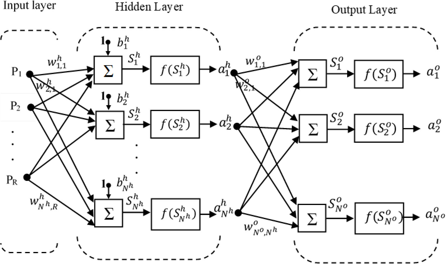
Figure 1.
ANN architecture
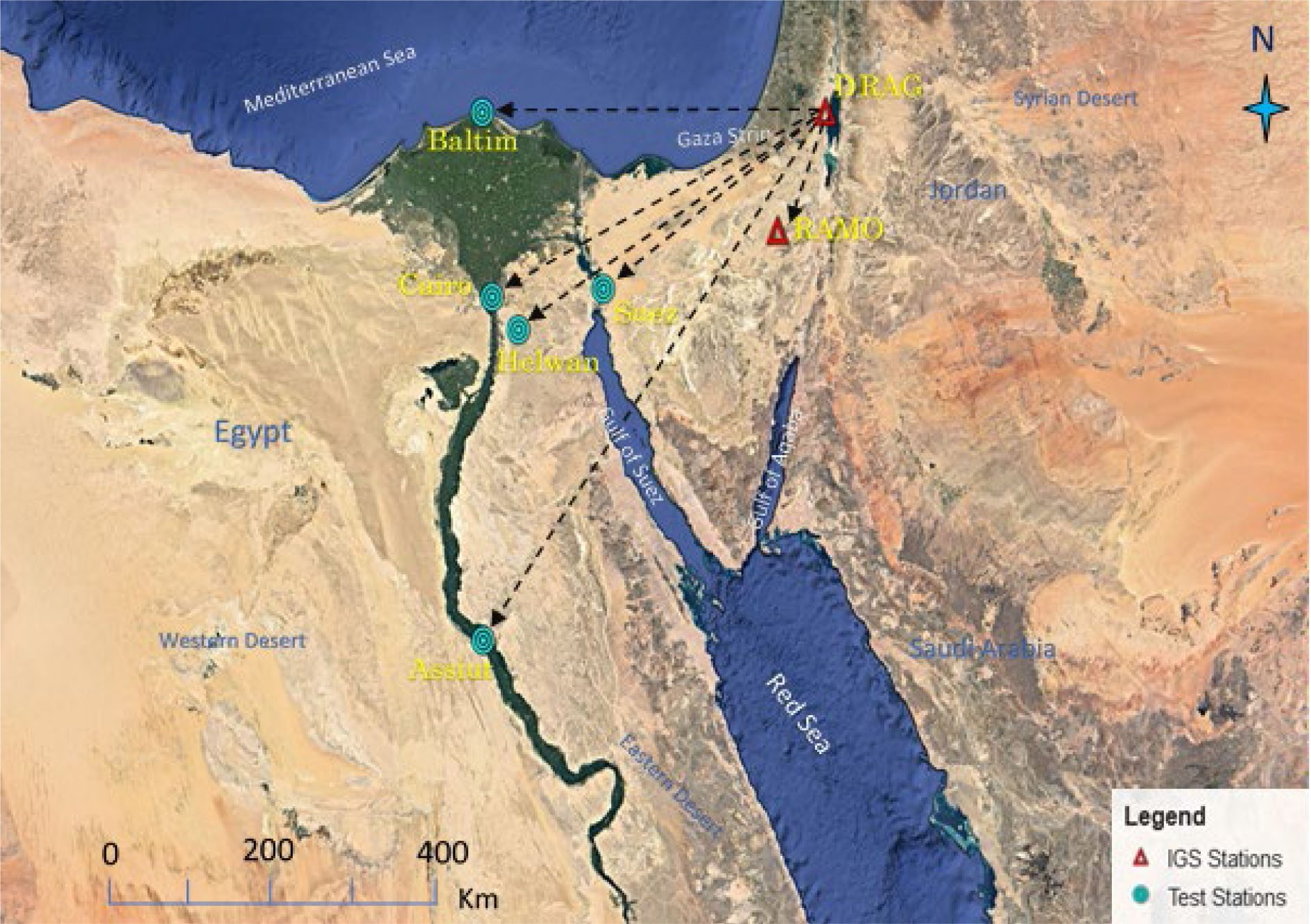
Figure 1.
Study area and IGS stations
Table 2.
Data sources
| Station | Station type | GNSS instrument | Reference coordinates | |||||||
|---|---|---|---|---|---|---|---|---|---|---|
| Longitude | Latitude | Ellipsoidal height, m | Source | |||||||
| ° | ′ | ″ | ° | ′ | ″ | |||||
| DRAG | IGS | Leica GRX1200 | 35 | 23 | 31.46180 | 31 | 35 | 35.5288 | 31.834 | SOPAC |
| RAMO | IGS | Leica RS500 | 34 | 45 | 47.31050 | 30 | 35 | 51.38602 | 886.829 | SOPAC |
| Baltim | Test | Trimble R8 | 31 | 04 | 49.15000 | 31 | 35 | 45.42070 | 31.163 | CSRS |
| Suez | Test | Trimble R8 | 32 | 36 | 22.45620 | 30 | 07 | 09.53080 | 53.827 | CSRS |
| Helwan | Test | Trimble R8 | 31 | 20 | 37.30370 | 29 | 51 | 33.72150 | 135.055 | CSRS |
| Cairo | Test | Leica GR10 | 31 | 14 | 16.45330 | 30 | 02 | 43.33490 | 68.268 | CSRS |
| Assiut | Test | Ashtech Z-Xtreme | 31 | 10 | 19.90010 | 27 | 11 | 12.12040 | 91.420 | CSRS |
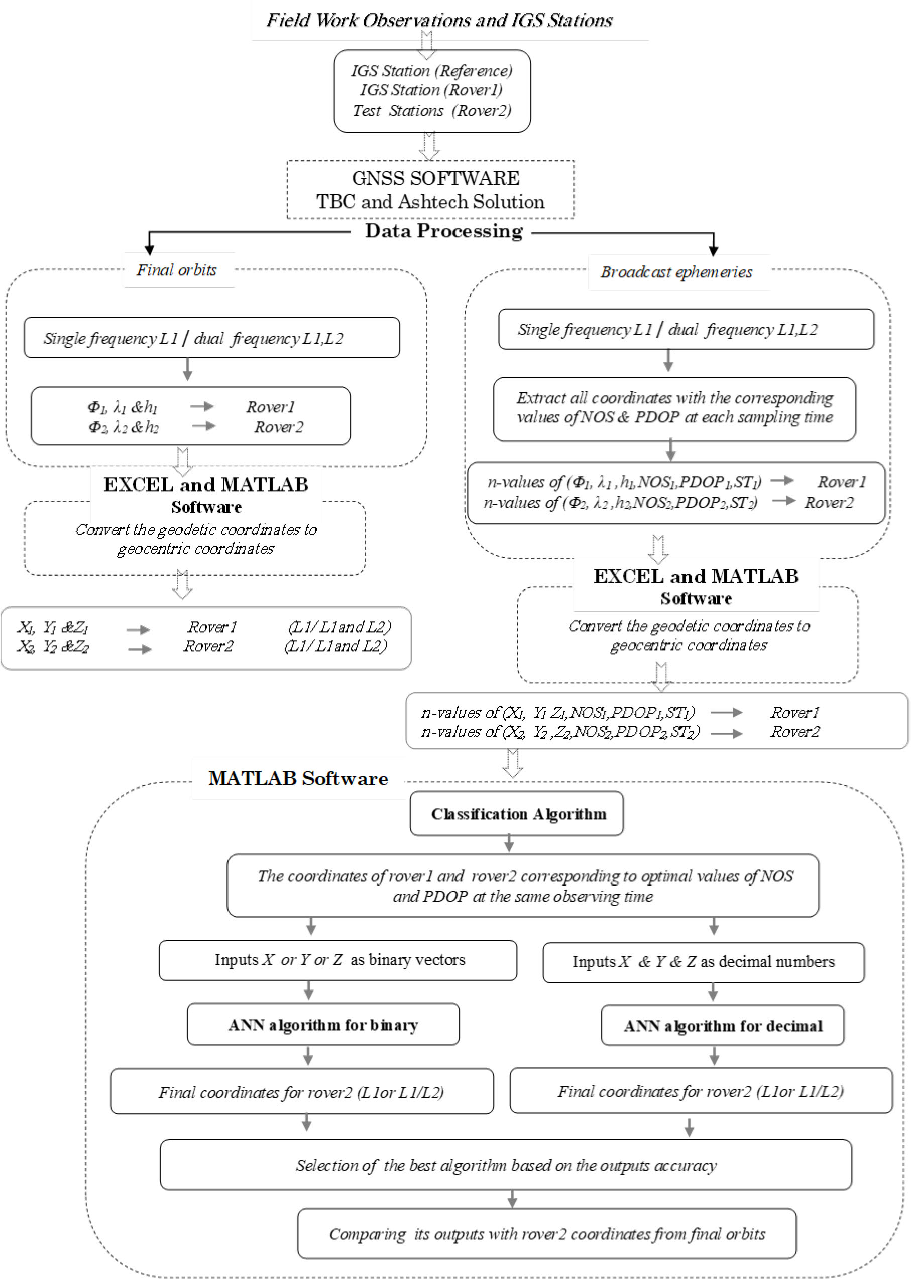
Figure 3.
Methodology flowchart
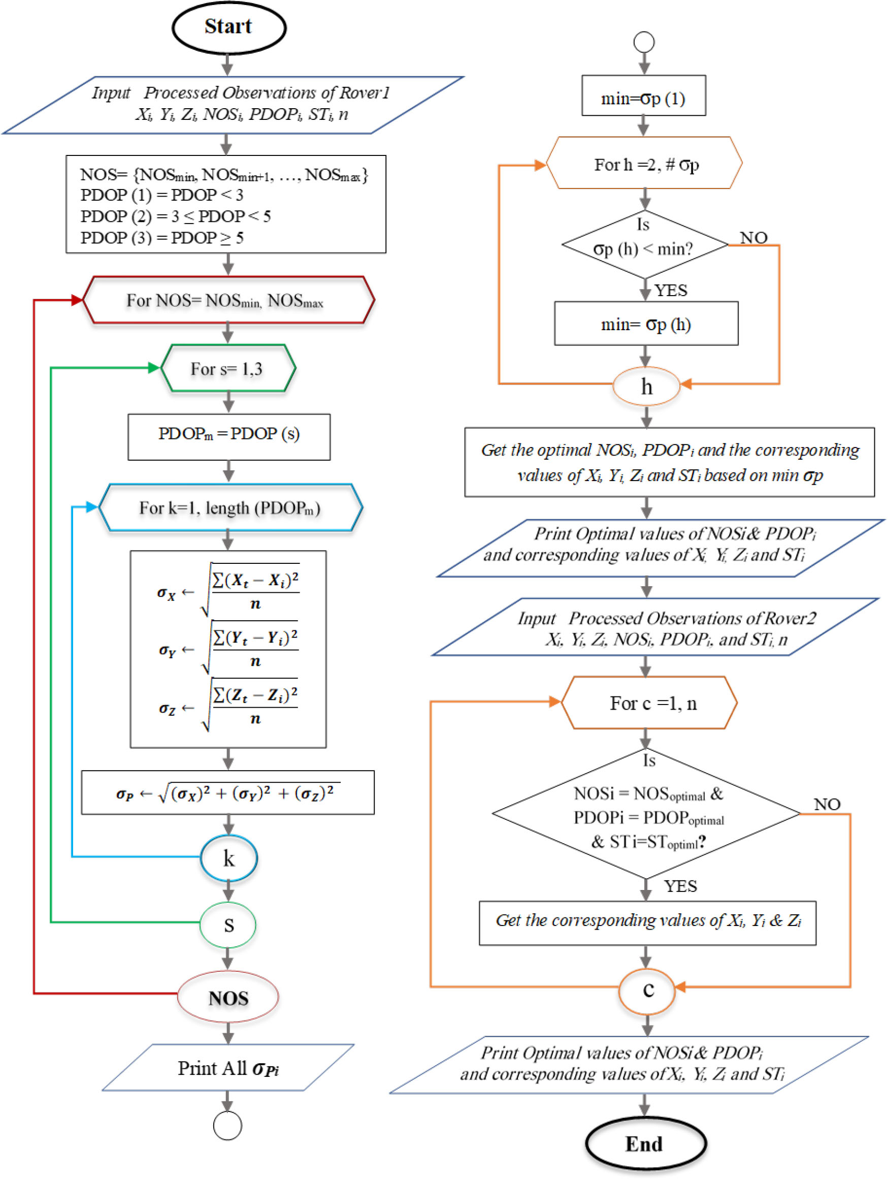
Figure 4.
Algorithm steps of the classification stage
Xi, Yi, Zi: coordinates values at each NOS, PDOP and ST
n: Number of the processed observations
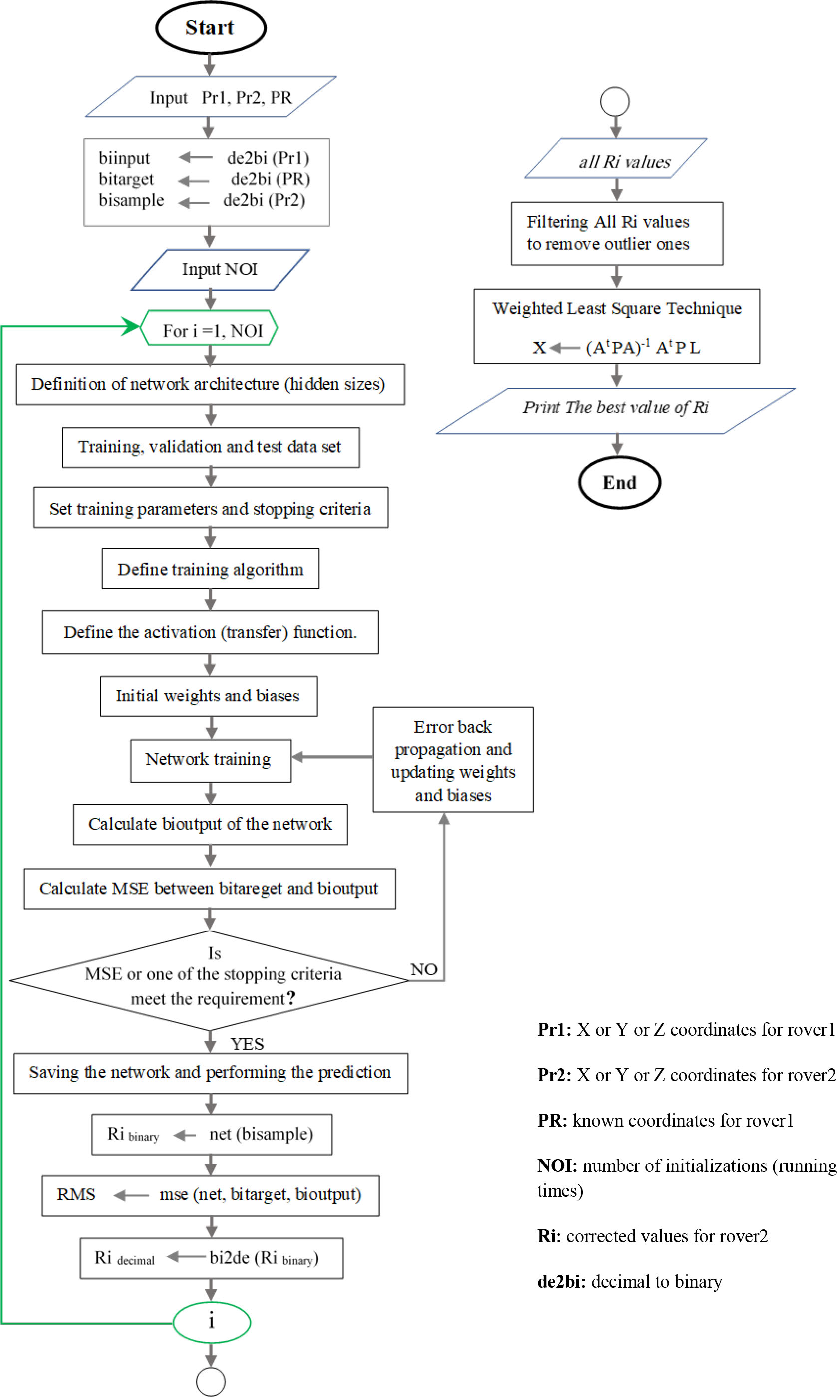
Figure 5.
Algorithm steps of the ANN stage (binary numbers)
Table 3.
The tested parameters in the ANN algorithm
| Test no. | Transfer function | ANN type | NHL | NON | NOI | |
|---|---|---|---|---|---|---|
| 1 | Transfer function | X | Fit net | 1 | 10 | 100 |
| 2 | ANN type | The optimal at test 1 | X | 1 | 10 | 100 |
| 3 | NHL | The optimal at test 1 | The optimal at test 2 | X | 10 | 100 |
| 4 | NON | The optimal at test 1 | The optimal at test 2 | The optimal at test 3 | X | 100 |
| 5 | NOI | The optimal at test 1 | The optimal at test 2 | The optimal at test 3 | The optimal at test 4 | X |
Table 4.
The parameters involved in the ANN algorithm
| Epoch | Goal | Max_fail | Min_fail | Mu | Learning rate |
|---|---|---|---|---|---|
| 1000 | 0 | 6 | 1e-7 | 0.001 | 0.01 |
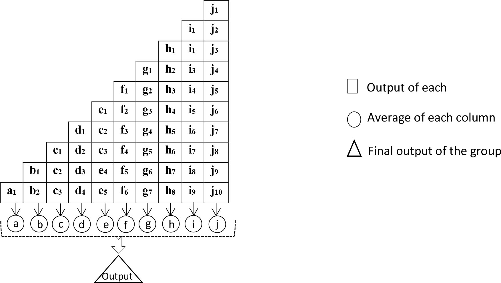
Figure 6.
A scheme displays the algorithm steps for producing reinitializing operation outputs (e.g., group 1)
Table 5 a-e.
The effect of different transfer functions’ constellation on ANN performance in the case of binary and decimal numbers (part 1/3)
| Transfer functions (hidden–output) layer | Binary numbers | |||||||||
|---|---|---|---|---|---|---|---|---|---|---|
| X | Y | Z | ||||||||
| σx (m) | MSE (m) | NOF | σY (m) | MSE (m) | NOF | σZ(m) | MSE (m) | NOF | ||
| a) Baltim station | Tansig–Purelin | 0.112 | 0.008 | 1 | 0.404 | 0.020 | 6 | 0.254 | 0.025 | 4 |
| Tansig–Logsig | NaN | NaN | 100 | NaN | NaN | 100 | NaN | NaN | 100 | |
| Tansig–Tansig | 0.103 | 0.005 | 2 | 0.319 | 0.007 | 7 | 0.050 | 0.003 | 5 | |
| Logsig–Purelin | 0.051 | 0.002 | 0 | 0.189 | 0.005 | 2 | 0.057 | 0.002 | 3 | |
| Logsig–Logsig | NaN | NaN | 100 | NaN | NaN | 100 | NaN | NaN | 100 | |
| Logsig–Tansig | 0.171 | 0.038 | 3 | 0.495 | 0.085 | 13 | 0.282 | 0.040 | 19 | |
| Purelin–Purelin | 1.048 | 0.094 | 7 | 0.955 | 0.087 | 2 | 0.489 | 0.054 | 6 | |
| Purelin–Logsig | NaN | NaN | 100 | NaN | NaN | 100 | NaN | NaN | 100 | |
| Purelin–Tansig | 0.537 | 0.041 | 7 | 0.805 | 0.049 | 6 | 0.669 | 0.085 | 7 | |
| Transfer functions (hidden–output) layer | Decimal numbers | |||||||||
| X, Y and Z | ||||||||||
| σx (m) | σy (m) | σz (m) | MSE (m) | NOF | ||||||
| Purelin–Purelin | 0.113 | 0.274 | 0.158 | 2 × 10⁻⁶ | 0 | |||||
| The other constellations of transfer functions | NaN | NaN | NaN | NaN | 100 | |||||
| b) Suez station | Transfer functions (hidden–output) layer | Binary numbers | ||||||||
| X | Y | Z | ||||||||
| σx (m) | MSE (m) | NOF | σY (m) | MSE (m) | NOF | σZ (m) | MSE (m) | NOF | ||
| Tansig–Purelin | 0.165 | 0.004 | 3 | 0.227 | 0.013 | 3 | 0.186 | 0.007 | 2 | |
| Tansig–Logsig | NaN | NaN | 100 | NaN | NaN | 100 | NaN | NaN | 100 | |
| Tansig–Tansig | 0.183 | 0.005 | 3 | 0.185 | 0.009 | 5 | 0.196 | 0.017 | 7 | |
| Logsig–Purelin | 0.095 | 0.002 | 1 | 0.133 | 0.005 | 0 | 0.117 | 0.001 | 1 | |
| Logsig–Logsig | NaN | NaN | 100 | NaN | NaN | 100 | NaN | NaN | 100 | |
| Logsig–Tansig | 0.245 | 0.021 | 7 | 0.401 | 0.005 | 6 | 0.293 | 0.004 | 6 | |
| Purelin–Purelin | 0.498 | 0.081 | 6 | 0.554 | 0.071 | 3 | 0.617 | 0.032 | 3 | |
| Purelin–Logsig | NaN | NaN | 100 | NaN | NaN | 100 | NaN | NaN | 100 | |
| Purelin–Tansig | 0.632 | 0.035 | 6 | 0.488 | 0.045 | 4 | 0.650 | 0.035 | 10 | |
| Transfer functions (hidden–output) layer | Decimal numbers | |||||||||
| X, Y and Z | ||||||||||
| σx (m) | σy (m) | σz (m) | MSE (m) | NOF | ||||||
| Purelin–Purelin | 0.171 | 0.206 | 0.256 | 3 × 10⁻⁸ | 1 | |||||
| The other constellations of transfer functions | NaN | NaN | NaN | NaN | 100 | |||||
Table 5 a-e.
The effect of different transfer functions’ constellation on ANN performance in the case of binary and decimal numbers (part 2/3)
| Transfer functions (hidden–output) layer | Binary numbers | |||||||||
|---|---|---|---|---|---|---|---|---|---|---|
| X | Y | Z | ||||||||
| σx (m) | MSE (m) | NOF | σY (m) | MSE (m) | NOF | σZ (m) | MSE (m) | NOF | ||
| c) Helwan station | Tansig–Purelin | 0.042 | 0.007 | 3 | 0.156 | 0.008 | 3 | 0.123 | 0.009 | 3 |
| Tansig–Logsig | NaN | NaN | 100 | NaN | NaN | 100 | NaN | NaN | 100 | |
| Tansig–Tansig | 0.065 | 0.005 | 5 | 0.192 | 0.012 | 5 | 0.099 | 0.004 | 5 | |
| Logsig–Purelin | 0.048 | 0.004 | 2 | 0.129 | 0.002 | 3 | 0.086 | 0.010 | 2 | |
| Logsig–Logsig | NaN | NaN | 100 | NaN | NaN | 100 | NaN | NaN | 100 | |
| Logsig–Tansig | 0.275 | 0.013 | 2 | 0.352 | 0.007 | 6 | 0.356 | 0.032 | 6 | |
| Purelin–Purelin | 0.520 | 0.027 | 4 | 0.581 | 0.035 | 4 | 0.492 | 0.009 | 7 | |
| Purelin–Logsig | NaN | NaN | 100 | NaN | NaN | 100 | NaN | NaN | 100 | |
| Purelin–Tansig | 0.452 | 0.008 | 5 | 0.611 | 0.041 | 5 | 0.470 | 0.036 | 5 | |
| Transfer functions (hidden–output) layer | Decimal numbers | |||||||||
| X, Y and Z | ||||||||||
| σx (m) | σy (m) | σz (m) | MSE (m) | NOF | ||||||
| Purelin–Purelin | 0.157 | 0.305 | 0.276 | 5 × 10⁻⁷ | 2 | |||||
| The other constellations of transfer functions | NaN | NaN | NaN | NaN | 100 | |||||
| d) Cairo station | Transfer functions (hidden–output) layer | Binary numbers | ||||||||
| X | Y | Z | ||||||||
| σx (m) | MSE (m) | NOF | σY (m) | MSE (m) | NOF | σZ (m) | MSE (m) | NOF | ||
| Tansig–Purelin | 0.143 | 0.007 | 4 | 0.031 | 0.010 | 3 | 0.133 | 0.008 | 2 | |
| Tansig–Logsig | NaN | NaN | 100 | NaN | NaN | 100 | NaN | NaN | 100 | |
| Tansig–Tansig | 0.127 | 0.001 | 3 | 0.108 | 0.008 | 4 | 0.186 | 0.015 | 3 | |
| Logsig–Purelin | 0.073 | 0.004 | 2 | 0.014 | 0.006 | 2 | 0.052 | 0.003 | 2 | |
| Logsig–Logsig | NaN | NaN | 100 | NaN | NaN | 100 | NaN | NaN | 100 | |
| Logsig–Tansig | 0.272 | 0.009 | 5 | 0.358 | 0.031 | 5 | 0.296 | 0.002 | 5 | |
| Purelin–Purelin | 0.382 | 0.012 | 4 | 0.399 | 0.023 | 3 | 0.488 | 0.047 | 7 | |
| Purelin–Logsig | NaN | NaN | 100 | NaN | NaN | 100 | NaN | NaN | 100 | |
| Purelin–Tansig | 0.484 | 0.023 | 6 | 0.511 | 0.045 | 5 | 0.388 | 0.071 | 4 | |
| Transfer functions (hidden–output) layer | Decimal numbers | |||||||||
| X, Y and Z | ||||||||||
| σx (m) | σy (m) | σx (m) | MSE (m) | NOF | ||||||
| Purelin–Purelin | 0.273 | 0.242 | 0.338 | 0.006 | 0 | |||||
| The other constellations of transfer functions | NaN | NaN | NaN | NaN | 100 | |||||
Table 5 a-e.
The effect of different transfer functions’ constellation on ANN performance in the case of binary and decimal numbers (part 3/3)
| Transfer functions (hidden–output) layer | Binary numbers | |||||||||
|---|---|---|---|---|---|---|---|---|---|---|
| X | Y | Z | ||||||||
| σx (m) | MSE (m) | NOF | σY (m) | MSE (m) | NOF | σZ (m) | MSE (m) | NOF | ||
| e) Assiut station | Tansig–Purelin | 0.219 | 0.008 | 3 | 0.327 | 0.010 | 1 | 0.530 | 0.016 | 6 |
| Tansig–Logsig | NaN | NaN | 100 | NaN | NaN | 100 | NaN | NaN | 100 | |
| Tansig–Tansig | 0.177 | 0.004 | 4 | 0.294 | 0.013 | 2 | 0.549 | 0.017 | 5 | |
| Logsig–Purelin | 0.149 | 0.006 | 2 | 0.225 | 0.007 | 0 | 0.481 | 0.015 | 5 | |
| Logsig–Logsig | NaN | NaN | 100 | NaN | NaN | 100 | NaN | NaN | 100 | |
| Logsig–Tansig | 0.314 | 0.009 | 5 | 0.470 | 0.023 | 4 | 0.640 | 0.022 | 7 | |
| Purelin–Purelin | 0.433 | 0.014 | 4 | 0.402 | 0.036 | 2 | 0.691 | 0.035 | 14 | |
| Purelin–Logsig | NaN | NaN | 100 | NaN | NaN | 100 | NaN | NaN | 100 | |
| Purelin–Tansig | 0.503 | 0.071 | 4 | 0.630 | 0.610 | 0 | 0.747 | 0.051 | 15 | |
| Transfer functions (hidden–output) layer | Decimal numbers | |||||||||
| X, Y and Z | ||||||||||
| σx (m) | σy (m) | σz (m) | MSE (m) | NOF | ||||||
| Purelin–Purelin | 0.259 | 0.301 | 0.606 | 0.003 | 7 | |||||
| The other constellations of transfer functions | NaN | NaN | NaN | NaN | 100 | |||||
Table 6.
The SD of X, Y, and Z coordinates, 3D position error, and elapsed time for three different types of ANN
| Station | Pattern net | Fit net | Cascade forward net | ||||||||||||
|---|---|---|---|---|---|---|---|---|---|---|---|---|---|---|---|
| σx (m) | σY (m) | σZ (m) | σP (m) | Elapsed time (s) | σx (m) | σY (m) | σZ (m) | σP (m) | Elapsed time (s) | σx (m) | σY (m) | σZ (m) | σP (m) | Elapsed time (s) | |
| Baltim | 0.090 | 0.263 | 0.071 | 0.287 | 44.4 | 0.056 | 0.219 | 0.030 | 0.228 | 38.8 | 0.043 | 0.188 | 0.021 | 0.194 | 27.9 |
| Suez | 0.078 | 0.118 | 0.157 | 0.211 | 47.3 | 0.072 | 0.101 | 0.106 | 0.163 | 36.2 | 0.077 | 0.099 | 0.103 | 0.162 | 24.4 |
| Helwan | 0.127 | 0.193 | 0.089 | 0.248 | 45.8 | 0.089 | 0.152 | 0.076 | 0.192 | 37.4 | 0.084 | 0.146 | 0.079 | 0.186 | 27.2 |
| Cairo | 0.161 | 0.068 | 0.118 | 0.211 | 46.9 | 0.115 | 0.044 | 0.066 | 0.140 | 35.1 | 0.084 | 0.029 | 0.048 | 0.101 | 28.9 |
| Assiut | 0.227 | 0.224 | 0.448 | 0.550 | 49.7 | 0.179 | 0.198 | 0.431 | 0.507 | 39.5 | 0.147 | 0.179 | 0.425 | 0.484 | 26.8 |
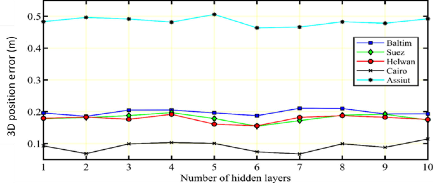
Figure 7.
The prediction error represented by the 3D position error versus the number of hidden layers
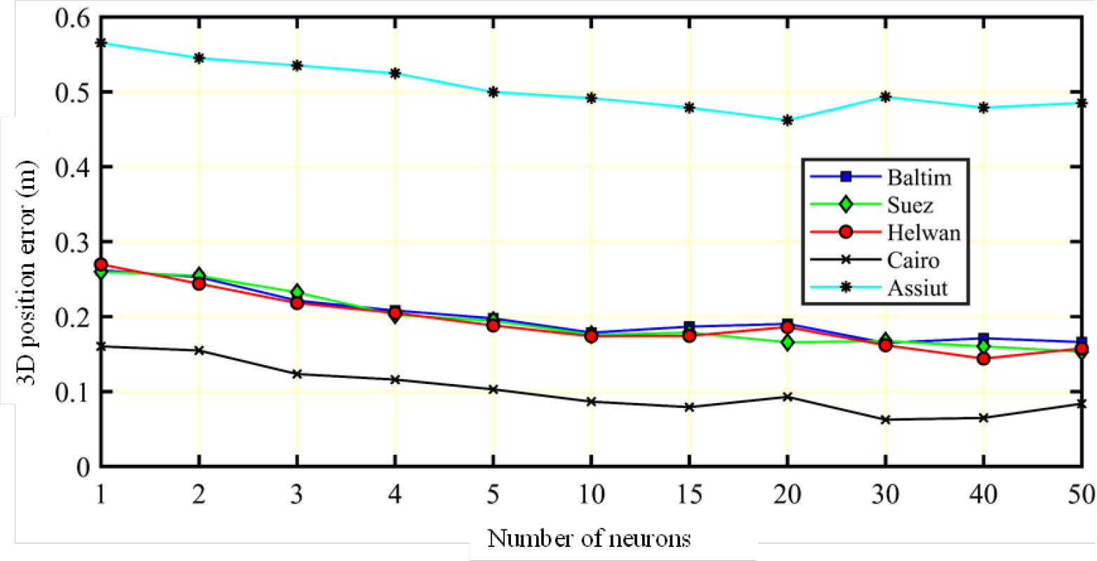
Figure 8.
The prediction error represented by the 3D position error versus number of neurons
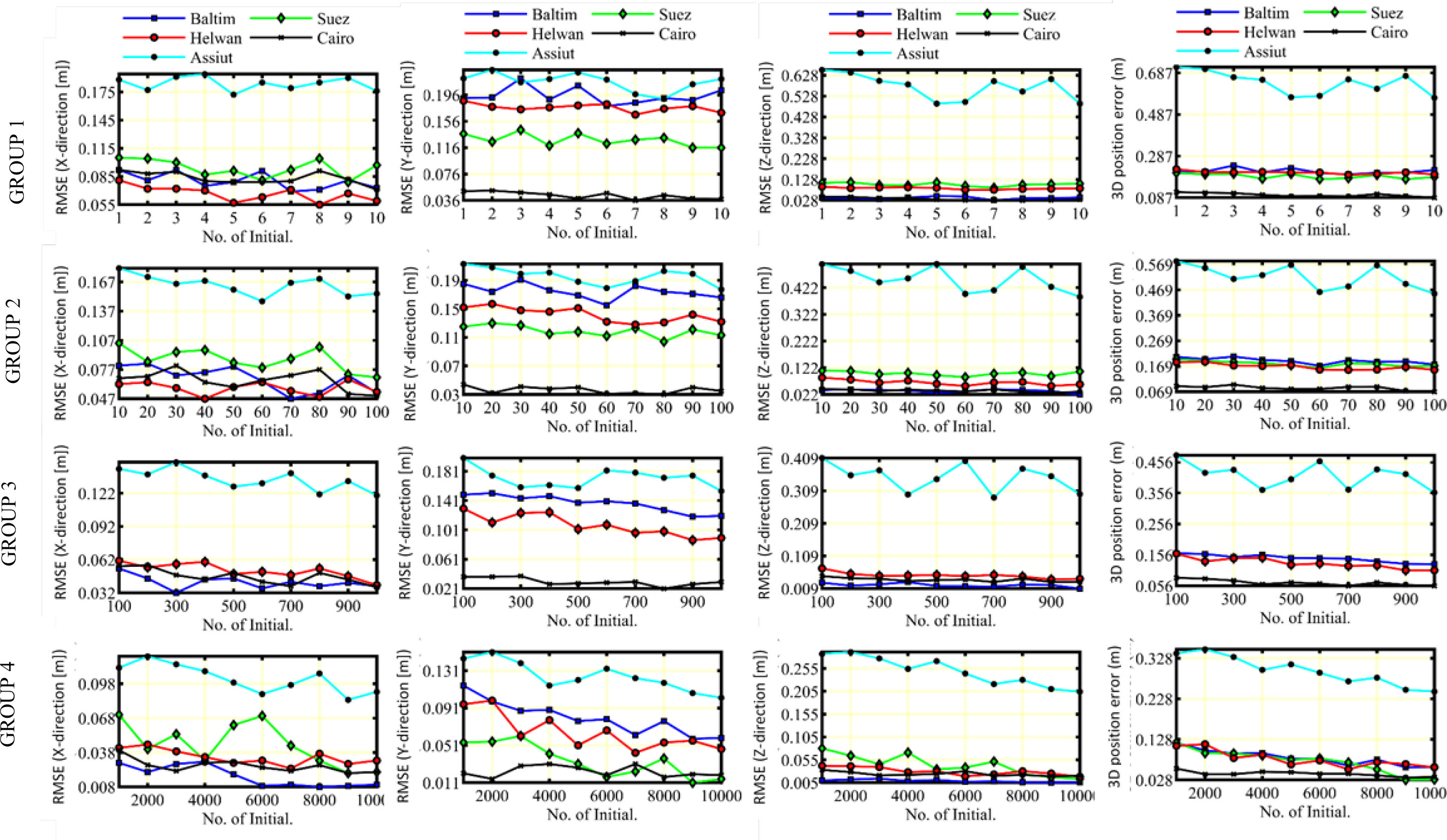
Figure 9.
RMSE of X, Y, and Z directions and 3D position error according to the different groups of the number of initializations
Table 7.
The averages of SDs in the directions of the coordinate axes, 3D position error, and elapsed time for the four groups of initialization numbers
| Station | Group 1 | Group 2 | Group 3 | Group 4 | ||||||||||||
|---|---|---|---|---|---|---|---|---|---|---|---|---|---|---|---|---|
| Nt values | Elapsed time (h) | Nt values | Elapsed time (h) | Nt values | Elapsed time (h) | Nt values | Elapsed time (h) | |||||||||
| 1–10 | 0.02 | 10–100 | 0.15 | 100–1000 | 1.5 | 1000–10,000 | 15.5 | |||||||||
| σm(X) (m) | σm(Y) (m) | σm(Z) (m) | σm(P) (m) | σm(X) (m) | σm(Y) (m) | σm(Z) (m) | σm(P) (m) | σm(X) (m) | σm(Y) (m) | σm(Z) (m) | σm(P) (m) | σm(X) (m) | σm(Y) (m) | σm(Z) (m) | σm(P) (m) | |
| Baltim | 0.080 | 0.195 | 0.040 | 0.215 | 0.068 | 0.174 | 0.036 | 0.191 | 0.042 | 0.137 | 0.019 | 0.145 | 0.017 | 0.080 | 0.009 | 0.083 |
| Suez | 0.094 | 0.128 | 0.105 | 0.190 | 0.087 | 0.119 | 0.101 | 0.179 | 0.068 | 0.085 | 0.082 | 0.137 | 0.045 | 0.035 | 0.044 | 0.074 |
| Helwan | 0.067 | 0.177 | 0.086 | 0.208 | 0.058 | 0.142 | 0.067 | 0.168 | 0.052 | 0.107 | 0.049 | 0.129 | 0.034 | 0.065 | 0.030 | 0.080 |
| Cairo | 0.083 | 0.044 | 0.035 | 0.100 | 0.066 | 0.036 | 0.036 | 0.084 | 0.047 | 0.030 | 0.036 | 0.066 | 0.026 | 0.023 | 0.024 | 0.043 |
| Assiut | 0.184 | 0.216 | 0.572 | 0.639 | 0.164 | 0.196 | 0.453 | 0.520 | 0.134 | 0.172 | 0.350 | 0.413 | 0.103 | 0.125 | 0.249 | 0.297 |
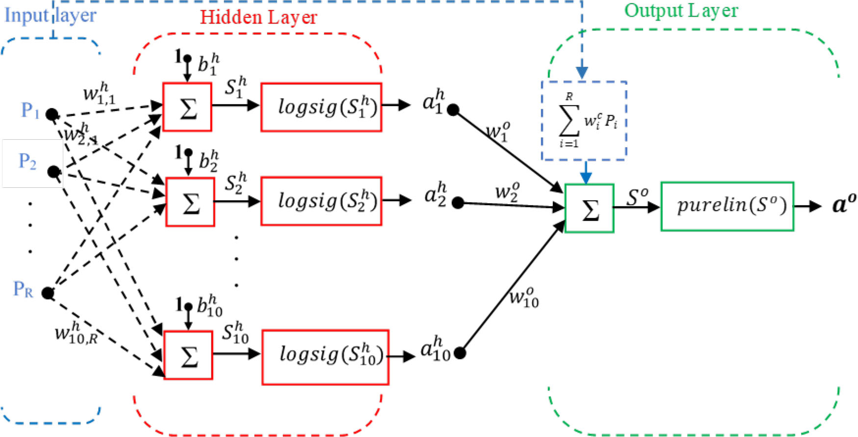
Figure 10.
The ANN designed from the results; its type is cascade forward net
Table 8.
The differences in coordinates between the known points and the output data, and the position errors for the three main stages in the case of GNSS-single frequency
| Station | Post-processing (broadcast ephemerides) | Classification algorithm | ANN algorithm | |||||||||
|---|---|---|---|---|---|---|---|---|---|---|---|---|
| dX (m) | dY (m) | dZ (m) | Position error (m) | dX (m) | dY (m) | dZ (m) | Position error (m) | dX (m) | dY (m) | dZ (m) | Position error (m) | |
| Baltim | 0.118 | 0.309 | 0.046 | 0.334 | 0.090 | 0.220 | 0.047 | 0.242 | 0.031 | 0.06 | 0.021 | 0.071 |
| Suez | 0.145 | 0.262 | 0.134 | 0.328 | 0.104 | 0.141 | 0.112 | 0.208 | 0.052 | 0.054 | 0.063 | 0.098 |
| Helwan | 0.123 | 0.277 | 0.204 | 0.365 | 0.075 | 0.190 | 0.092 | 0.224 | 0.078 | 0.081 | 0.051 | 0.123 |
| Cairo | 0.093 | 0.045 | 0.054 | 0.117 | 0.081 | 0.046 | 0.031 | 0.098 | 0.042 | 0.027 | 0.030 | 0.058 |
| Assiut | 0.286 | 0.330 | 0.992 | 1.084 | 0.190 | 0.241 | 0.675 | 0.741 | 0.101 | 0.132 | 0.381 | 0.416 |
Table 9.
The coordinates’ differences between the known points and the output data, and the position errors for the three main stages and IGS final orbits in the case of GNSS-dual frequency
| Station | Post-processing (broadcast ephemerides) | Post-processing (final orbits) | Classification algorithm | ANN algorithm | ||||||||||||
|---|---|---|---|---|---|---|---|---|---|---|---|---|---|---|---|---|
| dX (m) | dY (m) | dZ (m) | Position error (m) | dX (m) | dY (m) | dZ (m) | Position error (m) | dX (m) | dY (m) | dZ (m) | Position error (m) | dX (m) | dY (m) | dZ (m) | Position error (m) | |
| Baltim | 0.050 | 0.020 | 0.003 | 0.054 | 0.001 | 0.002 | 0.004 | 0.005 | 0.034 | 0.011 | 0.009 | 0.037 | 0.011 | 0.007 | 0.008 | 0.015 |
| Suez | 0.006 | 0.003 | 0.006 | 0.009 | 0.003 | 0.007 | 0.003 | 0.008 | 0.003 | 0.002 | 0.004 | 0.005 | 0.002 | 0.003 | 0.004 | 0.005 |
| Helwan | 0.047 | 0.040 | 0.019 | 0.065 | 0.015 | 0.015 | 0.011 | 0.024 | 0.024 | 0.021 | 0.024 | 0.040 | 0.017 | 0.016 | 0.021 | 0.031 |
| Cairo | 0.022 | 0.014 | 0.013 | 0.029 | 0.015 | 0.010 | 0.019 | 0.026 | 0.017 | 0.012 | 0.015 | 0.026 | 0.011 | 0.007 | 0.012 | 0.018 |
| Assiut | 0.157 | 0.051 | 0.322 | 0.362 | 0.044 | 0.083 | 0.110 | 0.145 | 0.103 | 0.062 | 0.220 | 0.251 | 0.051 | 0.021 | 0.153 | 0.163 |
Table 10.
Precision improvement due to applying classification and ANN algorithms in the two cases of observations
| Percentage of improvement (%) | ||||||
|---|---|---|---|---|---|---|
| Station | Single-frequency observations | Dual-frequency observations | ||||
| Classification algorithm | ANN algorithm | Classification algorithm | ANN algorithm | IGS final orbits | ||
| Baltim | 28 | 79 | 31 | 72 | 91 | |
| Suez | 37 | 70 | 44 | 44 | 11 | |
| Helwan | 39 | 66 | 38 | 52 | 63 | |
| Cairo | 16 | 50 | 10 | 38 | 10 | |
| Assiut | 32 | 62 | 31 | 55 | 60 | |