
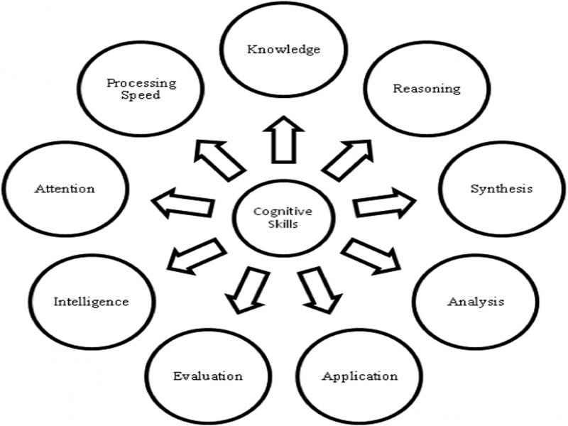
Figure 1:
Cognitive skills and related behaviors.
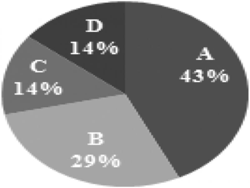
Figure 2:
Cognitive skill percentages for grade.
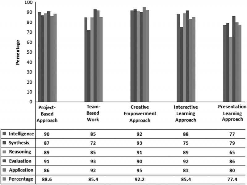
Figure 3:
Analysis of learning with various approaches.
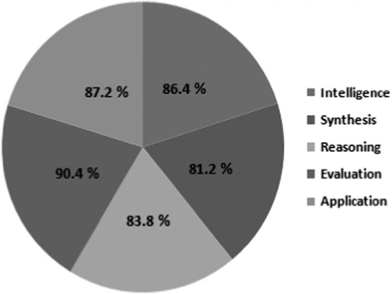
Figure 4:
Overall percentage of cognitive skills when applied with various learning approaches in an instructor-led virtual classroom.
Table 1.
Discriminant analysis for performance.
| Sample summary | Sample size | Internal 1 mean | Internal 2 mean | Attendance mean |
|---|---|---|---|---|
| Average | 5 | 54 | 51.2 | 89 |
| Good | 11 | 78 | 77 | 90.54545455 |
| Poor | 5 | 19.4 | 25.2 | 73.8 |
Table 2.
Classification matrix.
| Classification matrix | Average | Good | Poor | Correct |
|---|---|---|---|---|
| Average | 5 | 0 | 0 | 100 |
| Good | 3 | 8 | 0 | 72.7272727 |
| Poor | 1 | 0 | 4 | 80 |
Table 3.
Matrix of variance and covariance.
| Matrix of vars and covars | PA 1 | PA 2 | Attendance |
|---|---|---|---|
| Average | |||
| PA 1 | 126.5 | 243.5 | 96.5 |
| PA 2 | 243.5 | 472.7 | 178 |
| Attendance | 96.5 | 178 | 100.5 |
| Good | |||
| PA 1 | 258 | 163.6 | 10.4 |
| PA 2 | 163.6 | 152.2 | 7 |
| Attendance | 10.4 | 7 | 22.27273 |
| Poor | |||
| PA 1 | 237.8 | 190.4 | 126.85 |
| PA 2 | 190.4 | 268.7 | 107.8 |
| Attendance | 126.85 | 107.8 | 92.2 |
| Pooled | |||
| PA 1 | 224.289 | 187.31 | 55.41111 |
| PA 2 | 187.311 | 249.31 | 67.4 |
| Attendance | 55.4111 | 67.4 | 55.19596 |
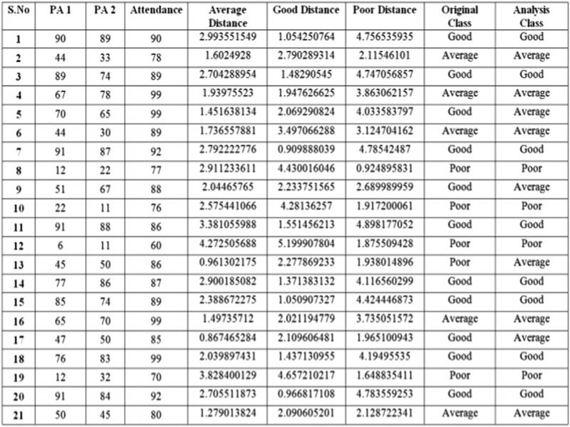
Figure 5:
Statistical distance of each observation to the mean vector.
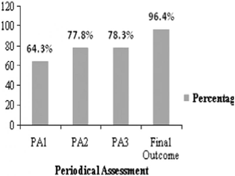
Figure 6:
Comparison of the final outcome with periodical assessment.
Table 5.
Summary statistics.
| Variable | Categories | Frequencies | % |
|---|---|---|---|
| Predicted performance | Average | 68 | 34.171 |
| Good | 62 | 31.156 | |
| Poor | 69 | 34.673 |
Table 6.
Summary statistics (validation).
| Variable | Categories | Frequencies | % |
|---|---|---|---|
| Predicted performance | Average | 0 | 0.000 |
| Good | 0 | 0.000 | |
| Poor | 1 | 100.000 |
Table 7.
Sum of weights and prior probabilities for each class.
| Class | Sum of weights | Prior probabilities |
|---|---|---|
| Average | 68.000 | 0.342 |
| Good | 62.000 | 0.312 |
| Poor | 69.000 | 0.347 |
Table 8.
Mahalanobis distances.
| Class | Average | Good | Poor |
|---|---|---|---|
| Average | 0 | 1,526.947 | 1,257.661 |
| Good | 1,526.947 | 0 | 2,554.130 |
| Poor | 1,257.661 | 2,554.130 | 0 |
Table 9.
Generalized squared distances.
| Class | Average | Good | Poor |
|---|---|---|---|
| Average | 2.147594 | 1,529.279 | 1,259.779 |
| Good | 1,529.094 | 2.332341 | 2,556.248 |
| Poor | 1,259.809 | 2,556.462 | 2.118397 |
Table 11.
P values for Fisher distances.
| Class | Average | Good | Poor |
|---|---|---|---|
| Average | 1 | 0.021 | 0.028 |
| Good | 0.021 | 1 | 0.006 |
| Poor | 0.028 | 0.006 | 1 |
Table 12.
Wilks’ Lambda test (Rao’s approximation).
| Lambda | 0.000 |
| F (observed value) | 7.018 |
| F (critical value) | 2.551 |
| DF1 | 384 |
| DF2 | 10 |
| P value | 0.001 |
| alpha | 0.05 |
Table 13.
Pillai’s trace.
| Trace | 1.992 |
| F (observed value) | 7.610 |
| F (critical value) | 2.310 |
| DF1 | 384 |
| DF2 | 12 |
| P value | 0.000 |
| alpha | 0.05 |
Table 14.
Hotelling–Lawley trace.
| Trace | 596.480 |
| F (observed value) | 7.256 |
| F (critical value) | 3.923 |
| DF1 | 384 |
| DF2 | 6 |
| P value | 0.011 |
| alpha | 0.05 |
Table 15.
Roy’s greatest root.
| Root | 426.213 |
| F (observed value) | 13.319 |
| F (critical value) | 3.691 |
| DF1 | 192 |
| DF2 | 6 |
| P value | 0.002 |
| alpha | 0.05 |
Table 16.
Eigenvalue.
| F1 | F2 | |
|---|---|---|
| Eigenvalue | 426.213 | 170.267 |
| Discrimination (%) | 71.455 | 28.545 |
| Cumulative % | 71.455 | 100.000 |
Table 17.
Bartlett’s test for eigenvalue significance.
| F1 | F2 | |
|---|---|---|
| Eigenvalue | 426.213 | 170.267 |
| Bartlett’s statistic | 1125.651 | 516.894 |
| P value | 0.000 | 0.000 |
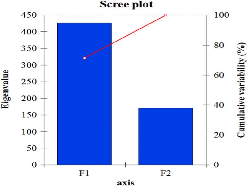
Figure 7:
Chart of the eigenvalue.
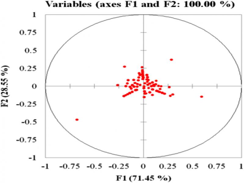
Figure 8:
Outcome of predicted performance with Bartlett’s test.
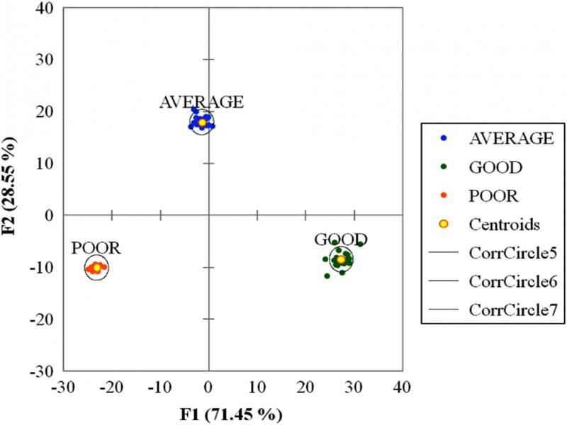
Figure 9:
Observations (axes F1 and F2: 100.00%).
Table 20.
Confusion matrix for the training sample.
| From/to | AVERAGE | GOOD | POOR | Total | % correct |
|---|---|---|---|---|---|
| AVERAGE | 68 | 0 | 0 | 68 | 100.00 |
| GOOD | 0 | 62 | 0 | 62 | 100.00 |
| POOR | 0 | 0 | 69 | 69 | 100.00 |
| Total | 68 | 62 | 69 | 199 | 100.00 |
Table 21.
Confusion matrix for the validation sample.
| From/to | AVERAGE | GOOD | POOR | Total | % correct |
|---|---|---|---|---|---|
| AVERAGE | 0 | 0 | 0 | 0 | 0.00 |
| GOOD | 0 | 0 | 0 | 0 | 0.00 |
| POOR | 0 | 0 | 1 | 1 | 100.00 |
| Total | 0 | 0 | 1 | 1 | 100.00 |
Table 22.
Confusion matrix for the cross-validation results.
| From\to | AVERAGE | GOOD | POOR | Total | % correct |
|---|---|---|---|---|---|
| AVERAGE | 23 | 26 | 19 | 68 | 33.82 |
| GOOD | 16 | 36 | 10 | 62 | 58.06 |
| POOR | 5 | 8 | 56 | 69 | 81.16 |
| Total | 44 | 70 | 85 | 199 | 57.79 |
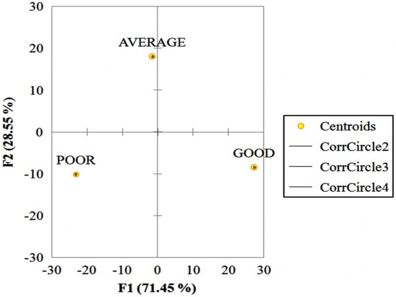
Figure 10:
Centroids (axes F1 and F2: 100.00%).