
Introduction
Researchers need to make decisions concerning sampling in each empirical study they are designing. In technology education research there are many sources of data, however the sample is often a cohort of students or teachers. Researchers may need to consider how representative the sample is of a population, whether a random sample is needed and/or viable as achieving this in educational research is particularly difficult, the feasibility of accessing the participants within a sample, and resources available (e.g., time, financial, personnel) to enable engagement with a sample.
Amongst these considerations, sample size is of critical importance. For qualitative researchers, such decisions often relate to saturation (Francis et al., 2010; Glaser & Strauss, 1967; Guest et al., 2006; Low, 2019) where the decision of when to stop collecting data is made during data collection. In contrast, for quantitative researchers the decision on how much data to collect should more typically be made before data collection begins. Outside of sequential designs where researchers intermittently check their data to see whether their results are statistically significant or not and use this as the basis for either stopping or continuing data collection (for a more detailed overview of sequential designs and optional stopping see Lakens, 2019; Lakens et al., 2023), quantitative researchers need to consider their sample size in advance of data collection to ensure they have enough statistical power to detect effects that exist within a population. Too low a sample size relative to a population effect size will result in a decreased probability to detect a real effect which can lead to researchers making a false negative inference. This can negatively impact the replicability of quantitative research, and has been observed in several fields including psychology (Open Science Collaboration, 2015), cancer biology (Errington et al., 2021), and economics (Camerer et al., 2016) among others. Implications of this include the basing of future research studies on findings which may lack credibility and validity, and translating such research into practice which could result in poor or negative practical implications within different fields.
In contrast, a study sample size could be considered excessively large and sub-optimal due to being a potential waste of resources. If, for example, for a given population effect a study design required a sample size of n = 100 to have a sufficiently high probability of detecting this effect, the collection of data from 1000 participants could be considered wasteful unless increased precision was deemed appropriate based on another criterion. A power analysis can be used to determine appropriate sample size requirements for different study designs based around the probability of detecting different population effect sizes. By increasing the probability of detecting true effects, researchers can reduce the probability of making false negative inferences.
A recent study indicated that the use of power analyses, or at least the reporting of any conducted power analyses, is limited in technology education research (Buckley, Araujo, et al., 2023). This may come from the use of rules of thumb or heuristic decision-making regarding sample sizes, or a lack of knowledge within the community regarding the use or value of power analyses, or of how to conduct them. Regardless, technology education research as a field does need to see improvements in replicability rates (Buckley et al., 2021; Buckley, Hyland, et al., 2023) which can come in part from increasing sample sizes to informed and pre-determined sizes. Therefore, this article will focus exclusively on providing a primer on how technology education researchers can determine minimum required sample size requirements for quantitative studies from this perspective. In doing so, this article will:
Describe the use of Cochran’s (1977) sample size formula to determine sample sizes for population representation in descriptive research,
Explain the concept of statistical power and the use of power analyses to determine minimum sample sizes in inferential studies,
Provide examples for conducting power analyses for studies employing the Pearson’s correlation and t-test tests, under the assumption of normally distributed data, as typical statistical tests used in technology education research.
Provide additional brief descriptions of the information needed for conducting power analyses for chi squared tests of independence, ANOVA models, and general linear models.
Discuss ways to determine population level effect sizes to use in statistical power calculations.
Determining sample sizes for population representation
Technology education researchers often ask descriptive research questions. For example, much research has been conducted aiming to describe attitudes towards technology in different geographical regions (cf. Ankiewicz, 2016). A researcher may, for example, seek to quantify the attitudes towards technology of a specific population. In such a study, access to the entire population is likely not feasible, and therefore the researcher would instead collect data from a sample with a view towards being able to generalize from this sample to the population. When designing a sample with the aim of being representative, researchers need to consider stratification and precision.
The creation of a stratified sample means constructing a sample which demographically reflects the population. To take a simplistic example, a hypothetical population of N = 100,000 may consist of 50,000 females and 50,000 males, i.e., an equal number of females and males. The researcher may therefore desire to create a stratified random sample by collecting data from an equal number of female and male participants. This process becomes more complex relative to the different demographic factors and levels within these factors that exist within the population which the researcher may need to account for. Technology education researchers often need to consider demographics such as gender, age, ethnicity, and socio-economic status, and thus the creation of a stratified random sample would include first determining the population demographic breakdown and then collecting data from a sample that is reflective and representative of this.
Once any decisions relating to the demographic breakdown of the sample are made, even if the decision is to not create a stratified sample, the researcher may then need to determine the number of participants from which to collect data. This decision may be for within demographic groups or for the whole sample depending on the nature of the study and the population the researcher is aiming to represent. Cochran’s (1977) sample size formula may be used for this as follows:
where no is the estimated sample size needed in situations where the total population size is unknown, z is the z-score corresponding to the confidence level desired (z = 1.96 for the often used 95% confidence level) with a higher z-score giving a higher confidence level and requiring a larger sample size, p is the proportion of the population estimated to have an attribute in question (0.5 is used to represent maximum variability [e.g., 50% of a population have a characteristic and 50% do not] and is thus often used in sample size calculations), and e is the desired margin of error (often 5% or 0.05) where a smaller value increases the required sample size due to increased precision.
If a total population size N is known or can at least be conservatively estimated, the no value can be then substituted into Equation 2 to calculate a required sample size n relative to that population size:
To put this into perspective, if a researcher was interested in collecting descriptive data from a population of N = 60,000, and they determined that this population was demographically broken down into two equally sized groups of 30,000, they may decide to randomly sample representative data from both groups. To achieve a sample with a 5% confidence interval at the 95% confidence level, the researcher would compute the sample size as 380 per demographic group to give a total sample size of n = 760, by:
The concept of statistical power
If a quantitative researcher is not asking a descriptive research question, but instead intends to test a specific directional or non-directional hypothesis, they need to consider associated error rates. In this paper two types of error will be primarily discussed, Type I and Type II errors. First, for any given hypothesis, within the population of interest there either is or is not an effect in reality. Assuming the entire population is not accessible, a sample is identified from which data is collected to test that hypothesis. The results of this test are then used to make an inference regarding the population.
To give context to this, as there is much research conducted on educational assessment in technology education (e.g., Bartholomew & Jones, 2021; Bartholomew & Yoshikawa-Ruesch, 2018; Buckley, Canty, et al., 2022; Buckley, Seery, et al., 2022), an example from this area will be given. For this example, a simplified account of the methodology implemented by Bartholomew et al. (2019) will be used1 and presented as though the study is in the planning stage. In their study, Bartholomew et al. (2019) implemented a quasi-experimental design to examine the effect of the use of adaptive comparative judgement (ACJ) (Hartell & Buckley, 2021) as a learning activity within a design task. A control and experimental group were formed, and both groups completed the same design activity. At the midpoint of the activity, the control group engaged in a traditional peer-sharing and feedback activity and the experimental group used ACJ in a process of providing feedback to their peers. The researchers sought to examine the effect of using ACJ in this way in comparison to the traditional peer sharing and feedback activity.
Considering this study as a potential investigation there are two possibilities in reality: there either is or there is not an effect of the use of ACJ in comparison to traditional peer-sharing and feedback. Following the completion of an empirical study to examine this hypothesis with a sample of participants, the results will either suggest that the null hypothesis of there being no effect should be rejected or accepted. Based on this, an inference can be made from the sample regarding the population (Table 1).
Table 1
Type I and Type II errors.
| Reality | |||
| Ho is true: no difference between ACJ and traditional peer sharing and feedback | Ho is false: there is a difference between ACJ and traditional peer sharing and feedback | ||
| Result of statistical test within an empirical study of a sample | Evidence to reject Ho | False positive Type I error Probability = α | Correct decision True positive Probability = 1 – β |
| No evidence to reject Ho | Correct decision True negative Probability = 1 – α | False negative Type II error Probability = β | |
Assuming that there is no difference in reality, the results of the study could lead to either making a correct decision if their statistical test provided no evidence to reject the null hypothesis (typically based on a p-value being greater than a predetermined alpha [α] value which is usually set at α = 0.05) or an incorrect false positive if the test provided evidence to reject the null hypothesis (typically observed as p < 0.05). A false positive error is a Type I error, and its probability (α) is usually set by technology education researchers as α = 0.05. In other words, when set as α = 0.05 and researchers compare statistically derived p-values to this threshold they are accepting a 5% false positive risk within their test.
In contrast, if in reality there is a difference between the use of ACJ and traditional peer-sharing and feedback, the result of the study could be statistically significant (typically p < 0.05) and lead to a correct inference by rejecting the null hypothesis, or it may not be significant (typically p > 0.05) and lead to an incorrect false negative inference. A false negative error is a Type II error, and its probability (β) varies based on the relationship between the α value, the statistical test, the population effect size, and the sample size. Given that the α value is typically a set value (e.g. α = 0.05), the statistical test would be planned based on the study design (e.g., a t-test), and the population effect size is generally unknown (but often estimated, which will be discussed later), researchers can affect the Type II error rate by adjusting their sample size. Specifically, increasing the study sample size increases statistical power (1 – β), which is the probability of rejecting a null hypothesis when it is false, or the probability to detect an effect with a sample that exists in reality in the population (Cohen, 1992). Such an increase thus reduces the probability of making a Type II, false negative, error (β) as there is more statistical power to detect an effect that does exist in the population or reality.
Conducting power analyses for t-tests and Pearson’s r statistical tests
Power analysis for t-tests
The previous example from the work of Bartholomew et al. (2019) can be used to illustrate the relationship between a study sample size and statistical power. In the example there are two groups, the control and experimental group, and the effect of ACJ in comparison to the traditional peer sharing and feedback activity was examined by comparing the performance of both groups in the design task. A t-test could be used in this example as a comparison of group mean difference. A power analysis could be performed at the planning stage to determine a minimum sample size for the study, and the researcher would need to make decisions on the significance criterion (α), a desired level of power (1 – β) or the probability they are willing to accept of not detecting a population level effect (β), and an estimate of a population level effect size (discussed later). Typically, a power analysis can be conducted with a software solution such as G*Power (Faul et al., 2007) or web app (which are free and require no knowledge of coding languages), but for this tutorial to explain further the concept of statistical power, simulations will be computed using R code. The full R code with associated outputs is available to view at https://osf.io/sc9pb/.
The following R code (Box 1) can be used to generate random data for two groups (hypothetically representative of the control and experimental groups from Bartholomew et al. (2019)). Specifically, the code defines two groups of n = 100 each, where the groups were formed as normally distributed random (technically pseudo-random due to being generated by a reproducible algorithm) samples from populations with mean performance scores of 70 and 65 respectively and with standard deviation values for their performance of 15.
Box 1: R code to simulate random, normally distributed data for two groups.
1.   set.seed(4239)
2.
3.   group.1 <- rnorm(n = 100, mean = 70, sd = 15)
4.   group.2 <- rnorm(n = 100, mean = 65, sd = 15)
This data has been simulated to have an effect in reality. Specifically, the effect is a population level difference of 5. However, this would more typically be described by a standardized effect size. In this instance, the Cohen’s d effect size would be appropriate where d represents the mean difference in terms of pooled standard deviation (cf. Lakens, 2013). In this example, d = .33, as the mean difference (70 – 65 = 5) is one third of the pooled standard deviation (15). Were this being simulated in advance of planning a study, this would be akin to assuming a population effect size of d = 0.33. Given that this effect is a population level effect, a t-test between the two samples will either lead to a correct decision if a statistically significant result is observed, or a false negative decision if a non-significant effect is observed. A t-test was performed (Box 2) on the simulated data through the following R code:
Box 2: R code to conduct a t-test between the two simulated groups.
5. t.test(group.1, group.2, var.equal = TRUE)
The results indicate a statistically significant difference, t(198) = 3.1654, p < 0.05, meaning that in this case a correct decision was made about reality based on the data collected from the sample of n = 200.
However, while this individual instance resulted in a correct decision, it is important to determine the probability of the study leading to a correct decision. It is possible from within this population where there is an effect, that data could be collected from a sample where the effect is not observable. Understanding the probability of this occurring is important for two reasons. First, prior to the study, given the aim of quantitative research is often to make generalizations to reality or the population, having a high probability of observing a result that reflects reality, or the population level effect is important. Second, after a study, when a result is observed it is important to be able to critique this in terms of how probable it was to occur. To determine this probability, the exact same process described in Box 1 and Box 2 will be simulated to repeat 5000 times. This allows for a percentage of times a significant difference between two such groups would be observed through the use of a t-test, and thus for the probability of observing the effect to be determined under these circumstances. The reason 5000 is specified as the number of replications is arbitrary. A large number of replications is needed for precise calculation, and 5000 is simply selected here to achieve that need. For all following simulations, this value of 5000 will remain set as a number of replications (Box 3).
Box 3: R code to set the number of replications as 5,000.
6. n.replications <- 5000
In Box 4 a loop is created for the 5000 replications in which each time normally distributed samples for two groups are determined as before with the same population level performance values, a t-test is performed, and the p-values are extracted.
Box 4: R code to simulate 5,000 replications where data is simulated for two groups and a t-test is performed with d = 0.33 population mean difference and a sample size of n = 100 per group.
7.    sig.results <- c()
8.
9.    set.seed(4239)
10.
11.   for (i in 1:n.replications) {
12.
13.    group.1 <- rnorm(n = 100, mean = 70, sd = 15)
14.    group.2 <- rnorm(n = 100, mean = 65, sd = 15)
15.
16.    t <- t.test(group.1, group.2, var.equal = TRUE)
17.
18.    sig.results[i] <- t$p.value <= 0.05
19.   }
Of the 5000 iterations, a significant result was detected 3258 times (65.16% of the time). Therefore, in a study where d = .33 is a population level effect size, having a sample size of n = 200 with n = 100 in both the control and experiment groups would have a statistical power level of 65.16% as there was a 65.16% chance of detecting the effect.
The code can be simplified by specifying the mean of group 1 to be 0, and the standard deviations of both groups to be 1 (Box 5). Then, whatever the mean of group 2 is set to will be the same as a Cohen’s d effect size. This is because the Cohen’s d effect size describes mean differences between groups in terms of standard deviations.
Box 5: R code to simulate 5,000 replications where data is simulated for two groups and a t-test is performed with d = 0.3 population mean difference and a sample size of n = 100 per group.
20.   sig.results <- c()
21.
22.   set.seed(4239)
23.
24.   for (i in 1:n.replications) {
25.
26.    group.1 <- rnorm(n = 100, mean = 0, sd = 1)
27.    group.2 <- rnorm(n = 100, mean = 0.3, sd = 1)
28.
29.    t <- t.test(group.1, group.2, var.equal = TRUE)
30.
31.    sig.results[i] <- t$p.value <= 0.05
32.   }
In the example in Box 5, from the 5000 replications, a statistically significant result was observed 2773 times, suggesting that for an effect size of d = 0.3, using a t-test to compare two independent groups with 100 cases in each has a statistical power level of 55.46%.
If the sample size is increased, such as to 150 participants per group, there is increased capacity to detect the effect size. With 150 cases per group, a significant result was observed 3728 of the 5000 iterations, or 74.56% of the time (Box 6).
Box 6: R code to simulate 5,000 replications where data is simulated for two groups and a t-test is performed with d = 0.3 population mean difference and a sample size of n = 150 per group.
33.   sig.results <- c()
34.
35.   set.seed(4239)
36.
37.   for (i in 1:n.replications) {
38.
39.    group.1 <- rnorm(n = 150, mean = 0, sd = 1)
40.    group.2 <- rnorm(n = 150, mean = 0.3, sd = 1)
41.
42.    t <- t.test(group.1, group.2, var.equal = TRUE)
43.
44.    sig.results[i] <- t$p.value <= 0.05
45.   }
By adjusting this code to compare population level effects of d = 0, 0.2, and 0.3, and sample sizes of n = 100, 150, and 200 per group (Figure 1), it is possible to see that when there is no population level effect (d = 0, Figure 1 panels A-C), a significant result is observed 5% of the time regardless of sample size. This equates to the specified α value of 0.05 which indicates 5% false positive risk acceptance or a 5% Type I error rate. When there is a population level effect or an effect in reality (d = 0.2 or 0.3, Figure 1 panels D-I) it is clear that increasing the sample size leads to an increased probability of detecting the effect. It is also clear that when the effect is larger, a lower sample size is needed to achieve a desired level of statistical power. For example, for d = 0.2 a sample size of n = 200 per groups results in statistical power of 0.51 (Figure 1 panel F) whereas for d = 0.3 a sample size of n = 100 per group results in statistical power of 0.56 (Figure 1 panel G) with n = 200 per group (Figure 1 panel I) giving a 0.85 power level.
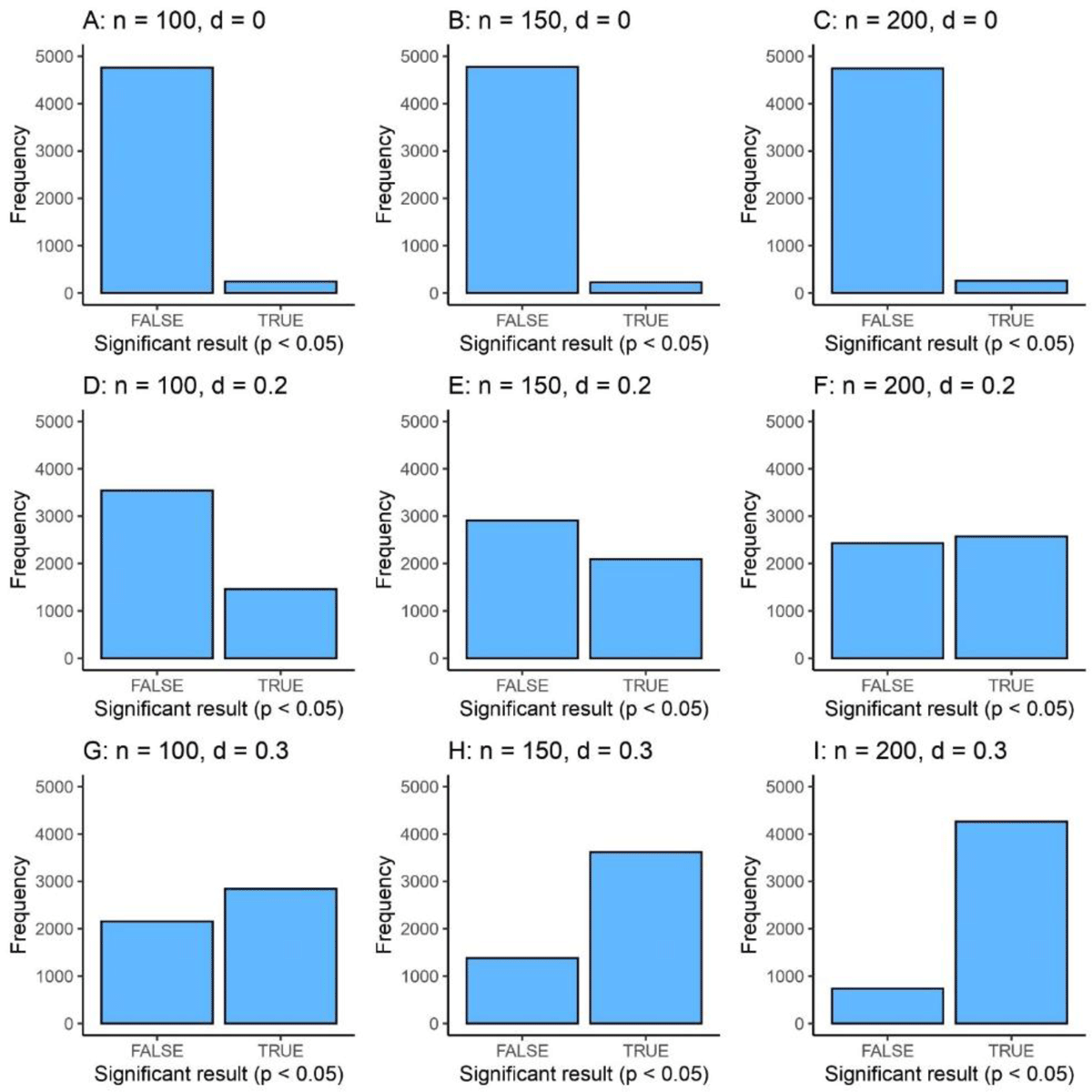
Figure 1
Results of power analysis for d = 0, 0.2, and 0.3 with n per group = 100, 150, and 200.
Power analysis for Pearson’s correlations
Statistical power can be computed the same way for research where correlation tests are planned. For this primer, statistical power calculations for the Pearson’s r correlation coefficient between two variables will be demonstrated.
Using the rnorm_multi() function in the faux R package (DeBruine, 2021), data for two variables can be simulated as collected from 50 cases. The mean of each variable is 0 and they both have standard deviations of 1. For the purposes of this example these are arbitrary and not relevant but are necessary for the code. The population level correlation specified is r = 0.3, and the variable names are “variable1” and “variable2” (Box 7).
Box 7: R code to simulate random, normally distributed data for 50 cases with two variables having a population level correlation of r = 0.3.
46.   set.seed(4239)
47.
48.   dataset <- rnorm_multi(n = 50,
49.                  vars = 2,
50.                  mu = 0,
51.                  sd = 1,
52.                  r = 0.3,
53.                  varnames = c("variable1", "variable2"))
Using the cor_test() function in the correlation R package (Makowski et al., 2020), a Pearon’s correlation test can be computed between these two simulated variables (Box 8).
Box 8: R code to conduct a correlation test between the two simulated variables.
54. cor_test(data = dataset, x = "variable1", y = "variable2", method = "pearson")
The result of this was that a statistically significant correlation was observed, r = 0.28, p < 0.05, within the sample, a result that would lead to the correct inference that there is an effect in reality within the population. However, this was just one instance, so as before a simulation study can be conducted similar to how one was conducted with the t-test (Box 9). The number of replications is consistent as 5000.
Box 9: R code to simulate 5,000 replications where data is simulated for two variables with a population correlation of r = 0.3 and a sample size of n = 50.
55.   sig.results <- c()
56.
57.   set.seed(4239)
58.
59.   for (i in 1:n.replications) {
60.
61.    dataset <- rnorm_multi(n = 50,
62.                   vars = 2,
63.                   mu = 0,
64.                   sd = 1,
65.                   r = 0.3,
66.                   varnames = c("variable1", "variable2"))
67.
68.    correlation <- cor_test(data = dataset, x = "variable1", y = "variable2", method = "pearson")
69.
70.    sig.results[i] <- correlation$p <= 0.05
71.
72.   }
A statistically significant correlation was observed 2850 times of the 5000 replications, or 57% of the time, illustrating 57% statistical power is achieved in studies where the population level effect size is r = 0.3 between two variables. If the sample size is increased to 70 participants for the simulation, a significant result is observed 3629 out of 5000 times, indicating that 72.58% power is achieved with this sample size for this population level effect size (Box 10).
Box 10: R code to simulate 5,000 replications where data is simulated for two variables with a population correlation of r = 0.3 and a sample size of n = 70.
73.   sig.results <- c()
74.
75.   set.seed(4239)
76.
77.   for (i in 1:n.replications) {
78.
79.    dataset <- rnorm_multi(n = 70,
80.                   vars = 2,
81.                   mu = 0,
82.                   sd = 1,
83.                   r = 0.3,
84.                   varnames = c("variable1", "variable2"))
85.
86.    correlation <- cor_test(data = dataset, x = "variable1", y = "variable2", method = "pearson")
87.
88.    sig.results[i] <- correlation$p <= 0.05
89.
90.   }
As with the t-test example, varying the effect size (r = 0, 0.2, and 0.3) and sample size (n = 50, 70, and 90) (Figure2) illustrates that (1) when there is no population level effect in reality (r = 0, Figure 2 panels A-C) a significant result is observed 5% of the time regardless of sample size as the α value used was 0.05, and that (2) when there is a population level effect (r = 0.2 or 0.3, Figure 2 panels D-I) statistical power is increased through the increasing of study sample size.
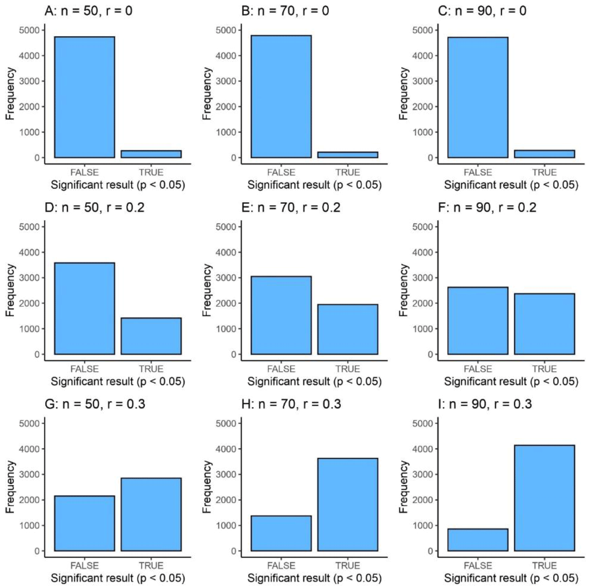
Figure 2
Results of power analysis for r = 0, 0.2, and 0.3 with n = 50, 70, and 90.
Conducting power analyses for common statistical tests in R and G*Power
For the most part, technology education researchers who plan to conduct a power analysis when designing their own studies do not need to simulate their data or write R code as above. The previous examples were presented as they were to be reproducible, to illustrate what is meant by a power analysis, and to demonstrate how to conduct such an analysis in the event that an easier tool is not available. There are now several user friendly shiny apps available for conducting power analyses for various types of research, including structural equation modelling (Jak et al., 2021), mediation analysis (Qin, 2023), factorial designs, (Lakens & Caldwell, 2021), and longitudinal designs (Lafit et al., 2021). These apps provide the capacity to enter relevant values relating to the study (e.g., the α value, desired statistical power, the number of variables, and effect sizes) outside of a code-based interface and based on the inputted information will output required sample sizes. The knowledge required by researchers is thus shifted from knowing how to simulate their study to understanding the input values and making decisions on relevant effect sizes.
However, it should be noted that these apps and software solutions which do not require writing code often require certain assumptions to be made. For example, many non-code-based applications assume that the sample is a random sample, and that the data are normally distributed. The prior simulations shown in this article also specify this through the use of the rnorm() and rnorm_multi() functions. An advantage of conducting a power analysis in a code-based environment is that different scenarios can be specified. While not shown here as this is meant to be an introductory primer, it would be possible to define the data as non-normal by, for example, adjusting skewness and kurtosis values. For any researcher intending to conduct a power analysis where such description is necessary or desired it may be useful to use a code-based simulation in the first instance.
Given that each of the previously cited shiny apps comes with an accompanying tutorial, and as this article is an introductory primer with the aim being that subsequent to engagement with this article technology education researchers will be equipped to engage with the wider variety of power analysis tools available, two introductory methods for basic power analyses reflecting common statistical tests used in technology education research will be demonstrated. The first is the pwr package in R (Champely, 2020) which has a series of functions that can be used to conduct power analyses without the need to simulate data. Six examples are given here for t-tests with equal sizes groups, t-tests with different sample sizes per group, r-tests, chi-squared tests, ANOVAs, and general linear models, but there are others available in the package. The second way does not require any knowledge of code, and that is to use the free G*Power software (Faul et al., 2007). This will be demonstrated only for t-test’s as the necessary information is consistent with that needed for the pwr package. G*Power also offers more functionality for different statistical tests that are not described here.
For each power analysis within the pwr package, certain information is needed. The pwr.t.test() function is used when a t-test is planned and the sample size would be the same between both groups. For this function, the input parameters are sample size per group (n), population level effect size (d), significance/α level (sig.level), power, the type of t-test as either two sample, one sample, or paired (type), and the nature of the alternative hypothesis as either a two sided non-directional test or a directional test. The function works by specifying one of these parameters as “NULL”, and that is the parameter which is then computed. If a researcher wanted to compute power achieved by a particular design they would specify the power parameter as NULL, but they could also set the sample size (n) parameter as NULL to determine a sample size required for achieving a particular level of power. For the below example (Box 11), setting the “power” parameter as NULL gives a result of power = 0.88, meaning that for a two-sided or non-directional two-sample or independent samples t-test with 80 participants per group and a population effect size of d = 0.5, 88% statistical power is achieved. In other words, there is an 88% chance of detecting this population level effect with this sample size.
Box 11: R code example of the pwr.t.test() function within the pwr package to compute statistical power.
91.   pwr.t.test(n = 80,
92.           d = 0.5,
93.           sig.level = 0.05,
94.           power = NULL,
95.           type = "two.sample",
96.           alternative = "two.sided")
If instead the two groups would be different in size, the pwr.t2n.test() function can be used with the only substantive difference being that both groups sample sizes (n1 and n2) are specified. With the example below (Box 12), power is calculated as 83% for a non-directional two group t-test with n1 = 80 and n2 = 60 when the population effect size is d = 0.5 and an α level of 0.05 is set.
Box 12: R code example of the pwr.t2n.test() function within the pwr package to compute statistical power.
97.   pwr.t2n.test(n1 = 80,
98.           n2 = 60,
99.           d = 0.5,
100.          sig.level = 0.05,
101.          power = NULL,
102.          alternative = "two.sided")
To use G*Power instead the interface would appear as in Figure 3. Here, the researcher first selects the statistical test they will perform, in this case a t-test to determine the mean difference between two independent groups, then selects the type of power analysis, which in this case is a priori to determine a required sample size, and then inputs the necessary information. In this example, it is shown that for a two-tailed non-directional t-test, with a population effect size of d = 0.5, an α value of 0.05, and equal group sizes, to achieve 80% power a total sample size of 128 is needed.
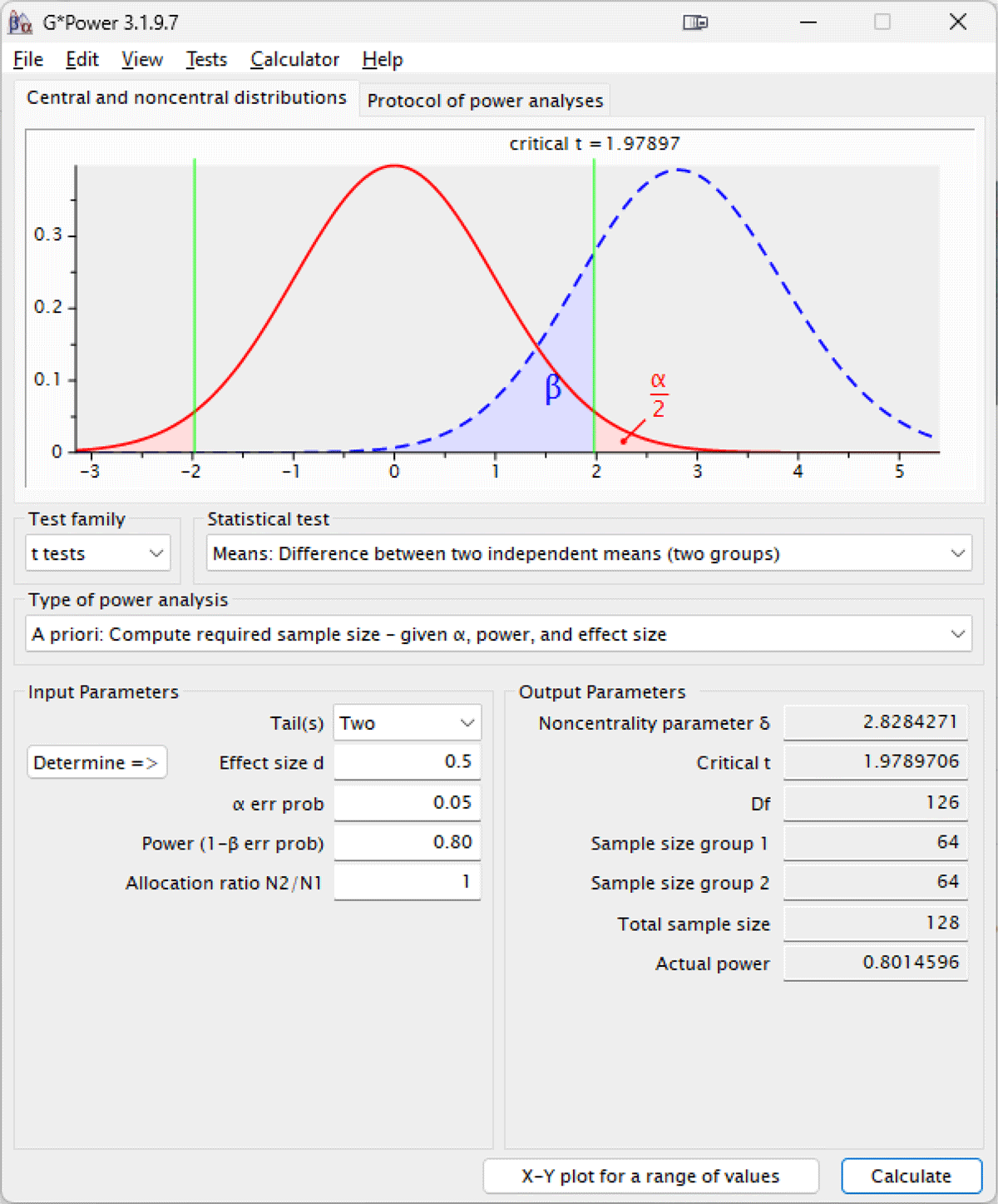
Figure 3
G*Power interface for conducting a power analysis for an independent samples t-test.
The pwr.r.test() function can be used to conduct a power analysis for use with the Pearson’s r correlation coefficient. Here, the researcher needs to consider sample size (n), the Pearson’s r correlation coefficient for the population effect size (r), significance/α level (sig.level), power, and the nature of the alternative hypothesis as either a two sided non-directional test or a directional test. Again, it may be more typical to leave the sample size as NULL and specify a desired level of power to determine a minimum sample size, but running the code in the below example (Box 13) shows that 96.2% power is achieved for a sample size of 80 in a two sided correlation test with an α value of 0.05 and population level effect size of r = 0.4.
Box 13: R code example of the pwr.r.test() function within the pwr package to compute statistical power.
103.   pwr.r.test(n = 80,
104.          r = 0.4,
105.          sig.level = 0.05,
106.          power = NULL,
107.          alternative = "two.sided")
For researchers who will use the chi squared test of independence, the pwr.chisq.test() function can be used. For this, they would need to understand the sample size (N), degrees of freedom (df) which equals the number of rows in the contingency table -1 multiplied by the number of columns in the contingency table -1, the Cohen’s W effect size (w), significance/α level (sig.level) and power. The example shown in Box 14 results in 77% power for the inputted parameters.
Box 14: R code example of the pwr.chisq.test() function within the pwr package to compute statistical power.
108.   pwr.chisq.test(N = 100,
109.           df = 2,
110.           w = 0.3,
111.           sig.level = 0.05,
112.           power = NULL)
If researchers are comparing more than 2 groups, which is often the case in technology education research, they would likely use a one-way ANOVA test. For this test, the pwr.anova.test() function can be used. Researchers need to input information on the number of groups (k), the sample size per group (n), the Cohen’s f effect size (f), significance/ α level (sig.level) and power. The example shown in Box 15 results in 77% power for the inputted parameters.
Box 15: R code example of the pwr.anova.test() function within the pwr package to compute statistical power.
113.   pwr.anova.test(k = 3,
114.           n = 40,
115.           f = .25,
116.           sig.level = 0.05,
117.           power = NULL)
A final example for this primer would be for researchers designing a study where they would analyze their data with a general linear model. In this case, they could use the pwr.f2.test() function and need to input information on the degrees of freedom for the numerator/number of predictor variables in the model (u), degrees of freedom for the denominator (v) which equals the sample size (n) – u – 1, the Cohen’s f2 effect size, significance/α level (sig.level), and power. The example in Box 16 indicates that for a linear model with 3 predictor variables (u) a sample size of 100 (v = n[100] -u[3] – 1), a significance level of α = 0.05, and a population effect size of f2 = 0.15, that 90.5% power is achieved in the overall model.
Box 16: R code example of the pwr.f2.test() function within the pwr package to compute statistical power.
118.   pwr.f2.test(u = 3,
119.           v = 96,
120.           f2 = 0.15,
121.           sig.level = 0.05,
122.           power = NULL)
Determining the population level effect size for use in power calculations
In most instances, power calculations are computed a priori. That is, they are computed at the planning stage to determine a minimum sample size requirement for a study to achieve a desired level of power relative to a population effect size. Typically, in the social sciences the desired level of power is 0.8 or 80% based on Cohen’s recommendation (Cohen, 1988). For reference, powering a study to 50% equates to an equal likelihood of detecting an effect that exists as not detecting it. Researchers can specify different levels of power, but when adopting this recommendation, the most pertinent question then becomes what effect size to power a study to. Going back to the design of the study of Bartholomew et al. (2019), if this was the study being planned, a two-tailed t-test was intended to compare the control and experimental groups of equal size, and the desired power was 0.8. With an alpha level of 0.05, and with an effect size of d = 0.5, the required sample size is n = 64 per group. However, if an effect size of d = 0.3 is used for the calculation the required sample size is n = 176 per group. The researcher needs to determine and justify the population level effect size they will power their study to.
A common perspective taken is to use effect size benchmarks. Cohen (1988) offered benchmarks for several effect sizes, such as for the Cohen’s d effect size as small (d = 0.2), medium (d = 0.5), and large (d = 0.8), and for the Pearson’s r effect size as small (r = 0.1), medium (r = 0.3), and large (r = 0.5). However, the intent was to use these only “when no better basis… [was] available” (p. 25). The issue with these benchmarks is that they are devoid of any reference. A “strong” correlation between two variables could have completely different practical meaning relative to a “strong” correlation between two other variables. Thus, powering a study to a “medium” effect (which appears common for the occasional usage of power calculations in technology education research) is problematic. Furthermore, this is not actually justification, as no explanation as to why a “medium” effect was selected is typically given.
A second common approach is to first conduct a pilot study to determine an effect size to use in a power calculation for a larger study. However, this again is problematic as the precision of a small sample pilot study to determine a population effect size is very low. The “corridor of stability” (Lakens & Evers, 2014) can be used to illustrate this reason. Figure 4 shows the results of three simulations.
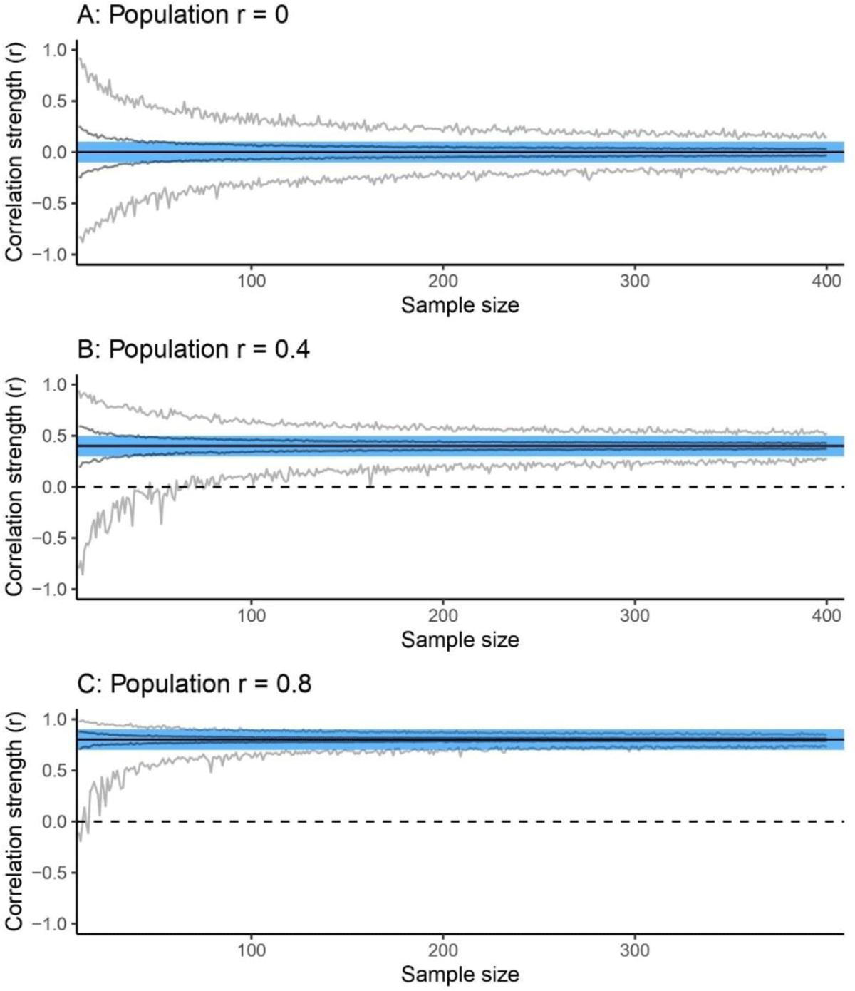
Figure 4
Sample size × effect size simulations.
In each, the population was defined as 60,000 people, and the population effect size (r) was set as r = 0, 0.4, and 0.8 between two random variables. For sample sizes of 10 to 400, 1,000 replications were conducted where a random sample of the data was “collected” and a correlation was computed between the two variables. The result (r) for smaller sample sizes is very often not close to the true population effect size, and unless the population effect size is quite large the pilot study outcome could often be in the opposite direction (different sign) to the population effect size. Using the results of a pilot study as an estimate of a population level effect size is likely to result in using an inaccurate effect size for the power calculation.
There are several options for how to determine a population effect size that can validly and justifiably be used. Funder and Ozer (2019) offer a list of approaches. One approach offered is to use benchmarking based on empirical works within the field. For example, researchers could use effect sizes based on classical studies within the field as benchmarks. For a technology education researcher, to give some examples, results from the e-scape project on educational assessment (Kimbell et al., 2005, 2007, 2009) or of the early work on attitudes towards technology (cf. Ankiewicz, 2016) immediately come to mind (although there are several more). Similarly, the use of other “well established” findings can be used as benchmarks. Another approach would be to compute average effect sizes coming from “all” technology education research studies. Such efforts have been made for social psychology (Richard et al., 2003) and could be emulated for technology education to determine field wide effect size estimates to use.
A second approach described by Funder and Ozer (2019) is to consider the consequences of effect sizes. This is described by Lakens (2021) as the smallest effect size of interest (SESOI). For example, if a technology education researcher were developing a pedagogical intervention aiming to increase student learning relative to a business as usual approach, this will require an investment of effort in implementation. If there is a resource cost in terms of time (e.g., the unit of learning in a business as usual case takes approximately 4 weeks, but the intervention approach takes 6 weeks) a cost benefit analysis would be useful. In such a case, it may be determined that a certain minimum effect size describing improved educational outcomes is needed to justify the increased time demands. In the case of Bartholomew et al. (2019), the intervention was the use of ACJ. This has a financial cost relative to the free peer sharing and feedback approach. Here, to justify the financial cost of ACJ integration into regular classroom practice it could be possible to justify a SESOI in the conduction of futher similar studies. The conversation on justifying a SESOI is expanded by Lakens et al. (2018).
Conclusion
The use of power analyses is rare in technology education research, but it is an important development to consider in future works to increase the replicability of research within the field (Buckley, Hyland, et al., 2023). Power analyses have limitations and researchers should not assume that achieving a desired level of power alone is sufficient to validate their sample. For instance, and as discussed already, the sample may be an adequate size but may be biased in other ways such as towards a particular demographic, or there may be selection or survivorship bias effects. Increasing statistical power also does not account for false positive risks brought upon by questionable research practices such as p-hacking or by conducting several exploratory analyses without giving consideration for increasing family-wise error rates. Statistical power and the conduction of power analysis is one of several sample-related considerations to be made, but it is critical that researchers and readers of research are aware of the statistical probability of results from samples reflecting reality and population level effects. This article aimed to offer a primer to support researchers in conducting power analysis for common research designs in the field and for engaging with the concept of power analyses further if they are conducting alternative or more complex studies.
Importantly, while this article has emphasized increasing sample sizes, it is important to keep in mind that this is not often possible. Often, resource limitations prevent large scale studies, or samples may become opportunistically available. Conducting under-powered research is not necessarily problematic as long as statistical power is considered. If a small sample is what is available, researchers may be unable to achieve a desired level of power, but they can describe their sample size and the achieved power relative to population effect sizes to note the probability of statistical error in their results. Further, small sample size studies can be included in subsequent meta-analyses, and meta-research is seeing an increase in technology education research.
Building on this, there is now a need for researchers to consider power in quantitative technology education research, and to support cases where the SESOI is difficult to determine, there is need to invest efforts in determining population effect sizes to use in power calculations. More broadly, there is need to consider improvements to research credibility in general, which can come from improvements in other areas such as reproducibility, robustness, and transparency (Buckley, 2023). In terms of reproducibility, which relates to independent confirmation of findings through the reproduction of analytic procedures with the same input data, one advance as seen in other fields such as psychology, includes journals (e.g. Meta-Psychology ISSN: 2003–2714) implementing reproducibility checks during the peer review process. This may be an option at the journal level within technology education. A more immediate action may be a field wide reproducibility analysis. For example, the Multi100 project (Aczel et al., 2022) is currently in the process of re-analyzing the central results of 100 social science articles across the fields of economics, political science, criminology, management, sociology, psychology, and organizational behavior. A similar project at a suitable scale could be conducted in technology education if authors of original studies were agreeable to share their data for re-analysis. In terms of robustness there are several approaches being used in other fields which can be adopted in technology education. One would be to conduct a “many analyst” study where original study datasets are analyzed by different researchers making different analytic decisions to determine the impact that such decisions have on the results (Botvinik-Nezer et al., 2020; Hoogeveen et al., 2023; Silberzahn et al., 2018). Alternatively, researchers in their own original studies could conduct multiverse analyses on their data (Steegen et al., 2016). This type of analysis sees the researcher specify decisions such as independent and dependent variables, covariates, statistical model type, and demographic group breakdown, and seeing the results of analyses under different decisions. A result is said to be robust if its observation does not depend on arbitrary analytic decisions. These types of work are typically related to quantitative research, but can be translated for qualitative research by considering the impact of different researcher epistemologies and positionalities on data generation and interpretation. This is equally useful when considering the transferability of qualitative findings between contexts. Finally, research can be improved in terms of transparency. To this end there have already been advances in technology education research. Buckley, with colleagues, has conducted two investigations into how transparent qualitative (Buckley, Adams, et al., 2022) and quantitative (Buckley, Araujo, et al., 2023) research is within the field, and these have resulted in two rubrics which can be used by technology education researchers to guide their methodological reporting to improve transparency.
Open science statement
The R code with outputs from this manuscript are available open access at https://osf.io/sc9pb/.