
1 Introduction
Since the pioneering work of Keeling and Shertz (1992), measurements of the abundance of atmospheric O2 and CO2 have been used extensively for determining fluxes of carbon to and from the land biosphere and the oceans. The budgets for atmospheric O2 and CO2 can be written as
where n and t are number of moles and time, Fx is the flux of CO2 from reservoir x to the atmosphere, αff (is the global average oxidative ratio of fossil fuels, αB is the effective average oxidative ratio of the global net land carbon sink and Zocean describes the outgassing of O2 from the ocean due to warming. Fcem represents the CO2 source associated with the manufacture of cement. αFF varies with time but is roughly 1.4 and αB is around 1.1 (Keeling and Manning, 2014).
In this paper, we address two shortcomings of Eq. 1: It assumes that atmospheric O2 is the exclusive oxidant for fossil fuels, and it neglects industrial oxygen fluxes that are not directly linked to fossil-fuel usage. Metal refining violates both of these assumptions. For example, during the refining of iron and aluminium, fossil carbon is oxidized by the oxygen present in hematite, magnetite and alumina, rather than atmospheric O2. During the refining of copper sulfides, O2 is removed from the atmosphere, independent of fossil-fuels.
We quantify these effects and correct for them by introducing a term to Eq. 1:
This allows fossil fuel O2 losses to be handled as before, with the metal refining being treated as an effective additional source of O2 to the atmosphere. We then use industrial records to determine annual values of Zmetals since 1990. Note that Zmetals is only needed for O2 since the CO2 flux associated with metal production is already included in equations 2 and 3 in the Fff term.
We further show that O2 and CO2 fluxes associated with sulfur are already included conceptually (and approximately) in these budget equations.
We focus on iron, aluminium, copper, and sulfur for two reasons: They are used in great quantities by humanity, and their oxidative states change between extraction and end use. Consequently, they are the heretofore neglected species with the greatest likelihood of influencing the abundance of atmospheric O2.
In the sections that follow, we treat each species in turn. We briefly describe the path from raw material to refined product and then estimate the quantities of product. From these, we calculate effective fluxes of O2 to/from the atmosphere. In all cases, we focus exclusively on the raw materials that end up as product and ignore effective fluxes of O2 associated with oxidation or reduction of raw materials that are extracted but not refined, such as mine tailings. We conclude by comparing the effective fluxes from these industrial materials to other terms and uncertainties in the budget.
2 Iron
Iron is an abundant and accessible element, enormously useful in both pure form and alloyed with various other metals as steel. In 2021, world production of iron ore contained about 1.6 × 10¹²kg (Tuck, 2022a) of iron, most of which was used to manufacture steel. The ore had a value of roughly $260 billion USD prior to refining (Statista, 2022c). Iron production was more than 25 times as great (by mass) than the next most heavily produced metal: aluminium (Bray, 2020a). With this ubiquity comes the potential for significant fluxes of O2.
With iron, as with our other species, we determine these fluxes by comparing the oxidative states of the raw and processed materials and scaling by the amount of product. Note that in our accounting, we are not concerned with fluxes related to the energy required for production. These are captured in the Fff term in equations 1 and 2.
2.1 Production Chemistry
Iron and steel are produced primarily from the important iron-bearing minerals hematite and magnetite .
At present, the great majority of hematite is turned into iron by reacting the mineral with carbon monoxide in the presence of heat. This strips the oxygen off the iron and turns the CO into CO2. Although this process typically occurs in three steps, the net reaction is
The carbon in this process typically arrives as coke (derived from coal) which is then partially combusted to form CO.
As written, this reaction shows that 3 moles of O2 will be required for every 4 moles of iron produced. However, the central question is where the O2 that ends up in CO2 comes from. Of the 12 oxygen atoms released in CO2, 6 of them came from the hematite, effectively yielding a source of 3 moles of O2 to the atmosphere.
The “O2 source” nature of the process becomes clearer if we recogize that the Fff formulation of Eq. 1 assumes the oxidant for fossil fuels is exclusively atmospheric O2. If there is a non-atmospheric oxidant, the equation needs a correction term. In particular, in the reductive refining of metals, the ore itself oxidizes the carbon in the fossil fuel, yielding reduced metal and CO2 as the products with little or no atmospheric O2 required. Thus, Eq. 1 overestimates O2 loss (relative to CO2 production) whenever oxidized metals are refined using fossil fuel carbon.
As a specific example, consider only the hematite reduction:
This immediately shows that producing 4 moles of reduced Fe will release 3 moles of O2. No matter what the method of hematite processing, because the end product is fully reduced iron, the Fe:O2 ratio remains 4:3.
Magnetite is processed slightly differently, with Fe3O4 and CO reacting to yield FeO and CO2. The FeO is further reduced with CO to yield pure iron with the following net reaction:
Not surprisingly, the Fe:O2 ratio is 3:2.
2.2 Inventory
We use data from the US Geological Survey Mineral Yearbooks (Tuck, 2020a, b) to quantify the global annual production of iron ore from 1990 through 2018. Values are given in Table 1, including both hematite and magnetite. We convert mass of ore to moles of hematite and magnetite by assuming that 80% of the ore is hematite (Tuck, 2019), but as shown below our results are relatively insensitive to this assumption. Using the Fe:O2 molar ratios of 4:3 and 3:2 respectively yields the source of atmospheric O2 associated with pig iron production presented in Table 1. A time series of these values is shown in Figure 1.
Table 1
World production of iron and the associated effective release of O2 to the atmosphere, totalled for each calendar year. While the most likely mix of iron-bearing minerals is 80% hematite and 20% magnetite (by mole), we include other (extreme) scenarios as a sensitivity study. Data from Tuck (2020a).
| YEAR | WORLD PRODUCTION OF REDUCED IRON (Pg) | ANNUALLY INTEGRATED O2 SOURCE (Tmol) ASSUMING 80% HEMATITE | ANNUALLY INTEGRATED O2 SOURCE (Tmol) ASSUMING 50% HEMATITE | ANNUALLY INTEGRATED O2 SOURCE (Tmol) ASSUMING 95% HEMATITE |
|---|---|---|---|---|
| 1990 | 0.54 | 7.09 | 6.85 | 7.21 |
| 1991 | 0.52 | 6.80 | 6.57 | 6.92 |
| 1992 | 0.50 | 6.52 | 6.30 | 6.64 |
| 1993 | 0.50 | 6.52 | 6.30 | 6.63 |
| 1994 | 0.51 | 6.76 | 6.53 | 6.88 |
| 1995 | 0.55 | 7.24 | 7.00 | 7.37 |
| 1996 | 0.55 | 7.18 | 6.94 | 7.30 |
| 1997 | 0.59 | 7.68 | 7.42 | 7.81 |
| 1998 | 0.57 | 7.53 | 7.27 | 7.66 |
| 1999 | 0.56 | 7.35 | 7.10 | 7.48 |
| 2000 | 0.60 | 7.93 | 7.66 | 8.07 |
| 2001 | 0.59 | 7.73 | 7.46 | 7.86 |
| 2002 | 0.61 | 8.07 | 7.80 | 8.21 |
| 2003 | 0.64 | 8.41 | 8.13 | 8.56 |
| 2004 | 0.75 | 9.87 | 9.54 | 10.04 |
| 2005 | 0.84 | 11.07 | 10.69 | 11.26 |
| 2006 | 0.96 | 12.66 | 12.23 | 12.87 |
| 2007 | 1.07 | 14.05 | 13.57 | 14.29 |
| 2008 | 1.13 | 14.84 | 14.33 | 15.09 |
| 2009 | 1.09 | 14.31 | 13.83 | 14.56 |
| 2010 | 1.17 | 15.36 | 14.84 | 15.63 |
| 2011 | 1.24 | 16.28 | 15.73 | 16.56 |
| 2012 | 1.26 | 16.55 | 15.98 | 16.83 |
| 2013 | 1.34 | 17.60 | 17.00 | 17.90 |
| 2014 | 1.45 | 19.04 | 18.39 | 19.37 |
| 2015 | 1.46 | 19.17 | 18.52 | 19.50 |
| 2016 | 1.47 | 19.30 | 18.65 | 19.63 |
| 2017 | 1.50 | 19.70 | 19.03 | 20.03 |
| 2018 | 1.52 | 19.96 | 19.28 | 20.30 |
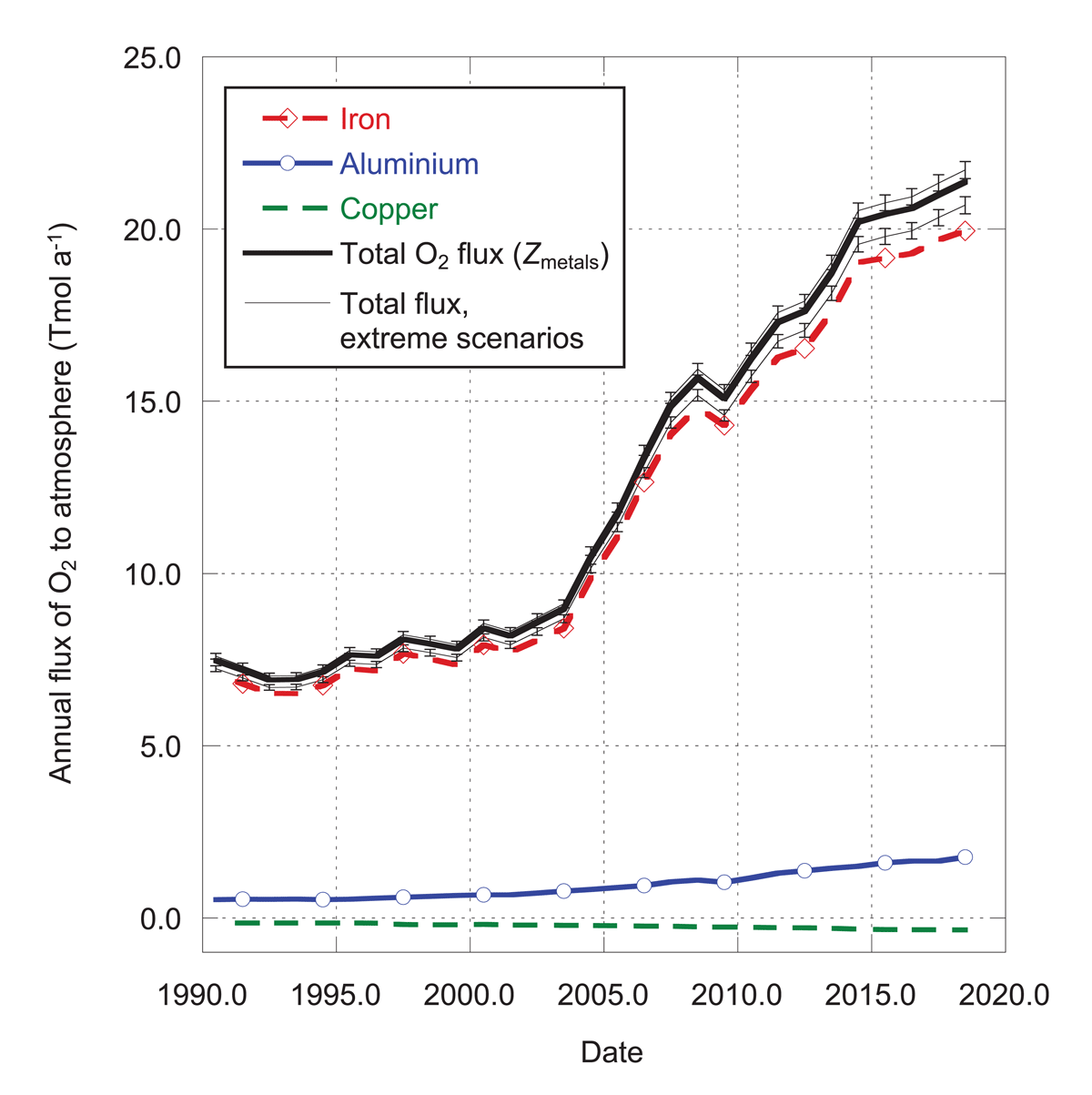
Figure 1
Effective fluxes of O2 to the atmosphere associated with production of various metals (1012 mol a–1). Negative values indicate a flux from the atmosphere. We assume iron is derived from 80% hematite and 20% magnetite (by mole). We assume copper is derived exclusively from sulfides. The heavy black line is the best estimate of total effective flux to the atmosphere from all sources (assuming an 80/20 mix of hematite and magnetite). The thin black lines show extreme cases (assuming 95% hematite and 50% hematite). Error bars on the extreme cases show the additional uncertainty (1σ) not originating from the unknown hematite/magnetite mix. Values are taken from Table 4, assigning the total annual value to the mid-year point and interpolating linearly.
The details of the fate of iron after it is mined are complicated, with various steps of concentration and refining yielding pig iron and ultimately steel. There are losses along the way, producing substantial quantities of slag and other byproducts. Nonetheless, effectively 100% of the oxidized iron extracted from the earth is reduced (Tuck, 2021), enabling the calculation of the atmospheric O2 source given above.
In practice, pig iron contains small amounts of carbon, sulfur, silicon, phosphorus and manganese; impurities that are removed as the pig iron is refined into steel. The dominant impurity is carbon, but since it enters the iron from coking coal during smelting its oxidation has been correctly captured by Fff in Eq. 1. Sulfur impurities are also almost entirely introduced by the coking coal, so their oxidation will be described by the treatment of sulfur in fossil fuels (see Sec. 5). Silicon is present in the ore in an oxidized state and remains so during smelting (SiO2 + CaO → CaSiO3). Phosporus and manganese are more complicated, as they are present in mineral ore in an oxidized state, are reduced early in processing, and are then re-oxidized at a later step. Thus, just as with silicon, phosphorus and manganese have no net O2 flux associated with processing.
We connect these production data to Zmetals by the Fe:O2 ratios given above. For example, if the world produces P moles of reduced iron in a time t and h% of that iron comes from hematite ore, the effective flux of O2 to the atmosphere will be where MFe is the molar mass of iron.
3 Aluminium
Aluminium, the third most abundant element in the earth’s crust, is a relative newcomer to human exploitation, first isolated in 1825 and widely used only after 1886 (Kesler and Simon, 2015). The demand for aluminium has grown steadily since then, due to its strength, light weight, and corrosion-resistance, leading to a commercial value second only to iron among metals. Global production in 2021 was 6.8 × 10¹⁰ kg (Bray, 2022) with a value of $170 billion USD (Statista, 2022a). Large as this is, the production is only 8% (by mole) of that of iron, implying a relatively modest impact on atmospheric oxygen.
3.1 Production Chemistry
Essentially all aluminium extracted for human use comes from bauxite, an ore containing various hydrated aluminium oxides, along with iron and other impurities. The primary oxides are diaspore and böhmite (both AlO(OH)), and gibbsite (Al(OH)3). About 85% of bauxite that is mined is converted to alumina (Al2O3) (Merrill, 2022) using the Bayer process of leaching and calcination. The abundances (both relative and total) of AlO(OH) and Al(OH)3 vary substantially from one deposit of bauxite to the next, but these two species have the same oxygen yields during refining. The remaining 15% of the bauxite is used for a variety of purposes but the aluminium in it is not reduced (Bray, 2021).
Of the alumina produced, the great majority (88% in 2017) (Bray, 2020a, b) is reduced to pure aluminium using the Hall-Heroult process. The remaining alumina is not further reduced, and is used instead in chemicals, abrasives and other products (Bray, 2021).
While the Bayer process (converting bauxite to alumina) is quite complicated, the net effect is a partial reduction of the hydrated oxides. Most importantly for our purposes, the liberated oxygen ends up as water. Thus, ignoring links between the oxygen and water cycles, the production of alumina has no impact on atmospheric O2.
In contrast, the reduction of alumina to aluminium using Hall-Heroult involves an electrochemical transfer of oxygen from the alumina to carbon from graphite anodes. The consequent release of CO2 is, once again, effectively a source of atmospheric O2 since there is oxidation of carbon with no impact on atmospheric O2 levels. Since the reduction of alumina can be represented as
the ratio of aluminium to O2 is 4:3.
3.2 Inventory
As with iron, we use data from the US Geological Survey Mineral Yearbooks (Bray, 2020a, b) for global annual production of pure aluminium from 1990 through 2017. Values are given in Table 2.
Table 2
World production of aluminium and the associated effective release of O2 to the atmosphere, totalled for each calendar year. Data from Bray (2020a, b).
| YEAR | WORLD PRODUCTION OF REDUCED ALUMINIUM (Tg) | ANNUALLY INTEGRATED O2 SOURCE (Tmol) FROM REDUCTION OF ALUMINA |
|---|---|---|
| 1990 | 19.3 | 0.54 |
| 1991 | 19.7 | 0.55 |
| 1992 | 19.5 | 0.54 |
| 1993 | 19.8 | 0.55 |
| 1994 | 19.2 | 0.53 |
| 1995 | 19.7 | 0.55 |
| 1996 | 20.8 | 0.58 |
| 1997 | 21.7 | 0.60 |
| 1998 | 22.6 | 0.63 |
| 1999 | 23.6 | 0.66 |
| 2000 | 24.3 | 0.68 |
| 2001 | 24.3 | 0.68 |
| 2002 | 26.1 | 0.73 |
| 2003 | 28.0 | 0.78 |
| 2004 | 29.9 | 0.83 |
| 2005 | 31.9 | 0.89 |
| 2006 | 33.9 | 0.94 |
| 2007 | 37.9 | 1.05 |
| 2008 | 39.7 | 1.10 |
| 2009 | 37.2 | 1.03 |
| 2010 | 41.8 | 1.16 |
| 2011 | 46.8 | 1.30 |
| 2012 | 49.3 | 1.37 |
| 2013 | 52.1 | 1.45 |
| 2014 | 54.1 | 1.50 |
| 2015 | 57.8 | 1.61 |
| 2016 | 59.5 | 1.65 |
| 2017 | 59.5 | 1.65 |
| 2018 | 63.6 | 1.77 |
| 2019 | 63.2 | 1.76 |
Since there is no O2 flux associated with the Bayer process, we only need to account for the refining of alumina to aluminium. Applying the 4:3 ratio given above yields the values shown in Table 2 as well as Figure 1.
4 Copper
Copper was one of the first metals used by humans and played a pivotal role in the development of civilization, first in pure form and later alloyed with tin as bronze. In modern society it remains essential, serving crucial functions in electrical power generation and electronics, plumbing, and marine applications. In 2021, roughly 2.1 × 10¹⁰ kg of copper was mined worldwide (Flanagan, 2022). This had a value of roughly $196 billion USD (Statista, 2022b). While these figures clearly show the global importance of copper, the production is only 1.1% of iron (by mole), suggesting a smaller influence on atmospheric oxygen than either iron or aluminium. The quantity of copper recycled and reclaimed is substantial (of order 5 × 10⁹ kg) but its processing does not generate O2 fluxes, so we ignore it in the work that follows.
4.1 Production Chemistry
The chemistry of copper production is more complicated than that of iron and aluminium since some copper-bearing minerals are sulfides while others are oxides. The dominant sulfides and their approximate fractional molar abundances are chalcopyrite (CuFeS2 70%), chalcocite (Cu2S 15%) and bornite (Cu5FeS4 10%). The oxides are primarily malachite (Cu2(CO3)(OH)2), atacamite (Cu2Cl(OH)3), brochantite (Cu4SO4(OH)6) and chrysocolla ((Cu,Al)2H2Si2O5(OH)4· nH2O), all roughly equally abundant (Sillitoe, 2021).
Sulfides account for about 85% of copper production (Schlesinger et al., 2011). Because the sulfides contain no oxygen, they cannot be a source to the atmosphere. Instead, the reduced sulfur and iron liberated during processing are eventually oxidized, functioning as a sink of atmospheric O2.
Elemental copper in chalcopyrite and bornite is extracted by concentration and smelting, followed by electrolytic refinement. The iron largely ends up in slag as FeO or Fe2O3 and the sulfur is emitted as gaseous sulfur dioxide (SO2). Copper in chalcocite is refined by leaching, followed by solvent extraction and electrowinning (SX-EW). This yields elemental sulfur. Regardless of the mineral type, the extraction method, or the intermediate oxidation state, the sulfur that is liberated nearly always ends up as sulfuric acid with three of the oxygen atoms in the H2SO4 coming from gaseous oxygen while the last comes from liquid water (Schlesinger et al., 2011). In the calculations that follow, as with aluminium we ignore any linkage between atmospheric O2 and the water cycle. For chalcocite this implies a sink of O2 in the molar ratio 4:3 (Cu:O2). For chalcopyrite and bornite, the ratios are 8:29 and 40:53 respectively, assuming equal amounts of ferric and ferrous oxide in the slag.
An additional complication for the sulfides is the risk of double-counting O2 fluxes associated with the oxidation of sulfur, since we develop a separate O2 budget for this element. We choose to include the O2 sink associated with copper sulfides in the copper budget rather than the sulfur budget, allowing us to limit the sulfur budget calculations to the reduced sulfur present in fossil fuels.
For the copper oxides, elemental copper is produced using the same methods employed for chalcocite, described above (leaching and SX-EW). The chemistry of the leaching is complicated by the variety of oxides to be considered and by the aqueous nature of the process. For example, when a single molecule of malachite is leached (by sulfuric acid), its five oxygens end up in one CO2 and three water molecules. Rather than try to account for the many possiblities, we simply ignore the small source of atmospheric O2 originating from processing of copper oxides, recognizing that oxides only account for 15% of copper production which is itself a small fraction of iron production.
4.2 Inventory
Again, we use data from the US Geological Survey Mineral Yearbooks (Flanagan, 2021) for global annual production of copper ore from 1990 through 2017. Values are given in Table 3.
Table 3
World production of copper and the associated removal of O2 from the atmosphere, totalled for each calendar year. We ignore copper produced from oxide minerals. We assume that 70% of the copper (by mole) comes from chalcopyrite, 15% from chalcocite and 10% from bornite (Sillitoe, 2021), with O2:Cu molar ratios of 29:8, 3:4 and 53:40, respectively. Production data from Flanagan (2021).
| YEAR | WORLD PRODUCTION OF REDUCED COPPER (Tg) | ANNUALLY INTEGRATED O2 SINK (Tmol) SULFIDES ONLY |
|---|---|---|
| 1990 | 8.62 | 0.15 |
| 1991 | 8.65 | 0.15 |
| 1992 | 8.73 | 0.15 |
| 1993 | 8.42 | 0.14 |
| 1994 | 8.43 | 0.14 |
| 1995 | 8.49 | 0.14 |
| 1996 | 9.05 | 0.15 |
| 1997 | 11.14 | 0.19 |
| 1998 | 11.40 | 0.19 |
| 1999 | 11.61 | 0.20 |
| 2000 | 11.02 | 0.19 |
| 2001 | 12.11 | 0.20 |
| 2002 | 12.19 | 0.21 |
| 2003 | 12.59 | 0.21 |
| 2004 | 12.81 | 0.22 |
| 2005 | 13.19 | 0.22 |
| 2006 | 13.73 | 0.23 |
| 2007 | 13.88 | 0.23 |
| 2008 | 15.03 | 0.25 |
| 2009 | 15.38 | 0.26 |
| 2010 | 15.85 | 0.27 |
| 2011 | 16.40 | 0.28 |
| 2012 | 16.88 | 0.29 |
| 2013 | 17.74 | 0.30 |
| 2014 | 19.20 | 0.32 |
| 2015 | 19.63 | 0.33 |
| 2016 | 19.96 | 0.34 |
| 2017 | 19.95 | 0.34 |
| 2018 | 20.27 | 0.34 |
We assume 85% sulfides, with the relative mineral species proportions (scaled to 100% abundance) and Cu:O2 ratios given above. Ignoring any O2 flux associated with the processing of oxides, we obtain the sink of atmospheric O2 given in Table 3 and shown in Figure 1. We recognize that ignoring oxides leads to a slightly exaggerated atmospheric O2 sink and discuss this further in Section 6.
5 Sulfur
Sulfur is widely used as an industrial raw material, and is essential in the world’s fertilizer and manufacturing sectors. The great majority of sulfur ends up as sulfuric acid, the most abundant inorganic chemical produced in the United States (Apodaca, 2022). The total world production of sulfur in 2017 was 80.2 million metric tonnes (Mt), slightly more than aluminium on a molar basis.
Significantly, only about 8% (as of 2017) of the world demand for sulfur is met by “discretionary” production, in which sulfur or iron sulfides (usually pyrite) are mined from discrete deposits (Apodaca, 2022). The remaining 92% of the world demand is met by “nondiscretionary” production: sulfur, sulfur dioxide and sulfuric acid recovered as byproducts of other process. The byproducts have significant commercial value and their abundance has led to almost complete cessation of Frasch-process sulfur mining (Ober et al., 2016).
The dominance of nondiscretionary production is a relatively recent phenomenon. Production of H2SO4 from fossil fuels began in the mid-1970s as regulation limited SO2 emissions. Global emissions of SO2 peaked at 130 Mt in the late 1980s and have fallen steadily since (Ober et al., 2016). The captured sulfur has almost completely replaced discretionary production. Globally, non-discretionary production now exceeds demand, driving down sulfur prices and leading to growing challenges for storage and disposal (Ober et al., 2016).
Thanks to this transition to non-discretionary production, sulfur is in a different category than iron, aluminium and copper: Current production of sulfur is almost entirely associated with fossil fuel production. This has two consequences. First, the sulfur in fossil fuels is in a reduced state and is subsequently oxidized, serving as a sink of atmospheric O2, much like the copper sulfides discussed above.
Second, we can largely incorporate sulfur directly into the O2 budget through careful handling of fossil fuel combustion with no need for separate O2 fluxes in Eq. 1. This was essentially done by Keeling (1988) when he used αff to characterize the fluxes of O2 associated with the combuston of non-carbon species present in fossil fuels. At the time of Keeling’s work, discretionary sulfur production was substantial. In the years since, it has become negligible, so Keeling’s formulation has the potential to completely account for the sulfur-driven sink of atmospheric O2. In brief, the value of αff is a consumption-weighted average of αgas, αliquid and αsolid. These fuel-specific oxidative ratios are built on the abundance of C, H, S & N in the fuels, assuming (among other things) the sulfur ends up as H2SO4. Thus, in Eq. 1, αff captures the O2 flux associated with all non-discretionary sulfur production.
In practice, this approach to budgeting has complications that are beyond the scope of this paper. For example, the chemistry of flue gas desulfurization changes both the O2 and CO2 fluxes somewhat. It is also possible that the amount of sulfur in the coal, oil and gas reserves currently being exploited is different from those in use nearly 40 years ago. Discretionary production of sulfur is not utterly negligible at 8% of the total. Some sulfur (perhaps 7% of production) is consumed as elemental sulfur (Messick, 2011), rather than being converted to H2SO4. Natural gas (essentially CH4) contains no sulfur, but is very often found with H2S. The latter is captured pre-combustion and converted to H2SO4, consuming O2. Additionally, correctly characterizing uncertainties is particularly challenging.
While we choose to defer a rigorous calculation, we can make a very rough estimate of the currently-neglected O2 sink associated with sulfur production. In 2017 world production of sulfur included 17 Tg from metallurgy, 49 Tg from liquid and gaseous fuels, 140 Tg from solid fuels and 13 Tg from sulfides and other discretionary production (Apodaca, 2022; Gilfillan and Marland, 2021; Keeling, 1988). If we assume each sulfur atom sinks 1.5 O2 molecules for solid fuels and 2.0 in every other case, this implies a sulfur-driven O2 sink of 11.5 Tmol in 2017. However, the αff formulation of Keeling (1988) takes nearly all of the O2 sink associated with the sulfur in liquid and solid fuels into account. Thus, taking the liquid and solid terms out of this total leaves 39 Tg (1.2 Tmol) of sulfur, removing 2.4 Tmol of O2 in 2017. We discuss the significance of this residual term in Sec. 6.2 below.
6 Results, Uncertainties and Discussion
6.1 Metals
Collectively, Tables 1, 2 and 3 show that the production of useful iron, aluminium and copper from mined minerals resulted in a net annual flux of O2 to the atmosphere of between 21 and 22 Tmol a–1 in 2017, depending on assumptions about the mix of iron species refined into metals. Averaged over the period 2000–2010, the range is 11.6–12.2 with a most likely value of 12.0 Tmol a–1. This flux (Zmetals) should be added into Eq. 1. Like all of the other terms in Eqs. 1 and 2, Zmetals varies over time. To facilitate incorporation of Zmetals in future O2-based carbon budgets, the total flux shown in Figure 1 is also given (with uncertainties) as Table 4. The uncertainty in these fluxes is difficult to rigorously quantify due to the assumptions involved in their estimation.
Table 4
Net effective oxygen release to the atmosphere associated with all metals for each calendar year (i.e. the annually integrated value of Zmetals). Units are 1012 moles (Tmol). Upper and lower uncertainties are the quadrature sum of the variations arising from the hematite/magnetite scenarios and all other errors.
| YEAR | ANNUALLY INTEGRATED O2 SOURCE (Tmol) |
|---|---|
| 1990 | |
| 1991 | |
| 1992 | |
| 1993 | |
| 1994 | |
| 1995 | |
| 1996 | |
| 1997 | |
| 1998 | |
| 1999 | |
| 2000 | |
| 2001 | |
| 2002 | |
| 2003 | |
| 2004 | |
| 2005 | |
| 2006 | |
| 2007 | |
| 2008 | |
| 2009 | |
| 2010 | |
| 2011 | |
| 2012 | |
| 2013 | |
| 2014 | |
| 2015 | |
| 2016 | |
| 2017 | |
| 2018 |
The largest uncertainty of which we are aware comes from the hematite/magnetite mix from which iron is refined. While an 80:20 (mol mol–1) mix is our best estimate, we only know with certainty that a majority of iron comes from hematite but some comes from magnetite. Thus, we consider 95:5 and 50:50 mixes as extreme cases around our 80:20 central value. These result in an asymmetric range of values for the estimated O2 flux from iron. In 2018, the effective oxygen release was .
Luckily, uncertain aspects of the processing of iron (e.g. losses to slag and other byproducts as iron ore becomes pig iron, or losses during transport) are irrelevant, as essentially 100% of the iron in the ore is reduced, regardless of whether it ends up in its intended form (Tuck, 2021).
We take the total production figures for iron, aluminium and copper from the USGS, which does not formally calculate uncertainties. Although presented by convention with three significant figures, the global values for iron production are likely good to 0.75% or better (Tuck, 2022c). Global copper production is significantly less certain (roughly 5% for solvent-extraction/electrowinning and 10% for primary smelting (Flanagan, 2022)). We assume similar uncertainty for aluminium (10%). For 2018, these imply uncertainties in the total effective release of O2 of 0.15, 0.03 and 0.18 Tmol of O2, respectively.
Our treatment of copper has several additional uncertainties and biases. We assume that iron present in copper sulfides is equally likely to be found in FeO and Fe2O3 states, but the true distribution is unknown. We assume an 85:15 split on copper sulfides and oxides, but do not know the uncertainty in that split. Lastly, we completely ignore the roughly 15% that are oxides because of the diversity of oxide minerals and the complexity of the processing. This omission will bias Zmetals low.
While our ignorance of uncertainties in copper production is unfortunate, it has little impact on the uncertainty in Zmetals simply because production of copper is so much smaller than production of iron. Even if the O2 fluxes from copper carry a 25% uncertainty (an arbitrary, but very conservative number, allowing for the production uncertainty given above and 23% uncertainty from other sources), the 2018 O2 consumption due to processing of copper will be known to ± 0.09 Tmol.
Uncertainty in O2 fluxes from aluminium are driven entirely by uncertainties in production so the value of 0.18 Tmol of O2 (for 2018) quoted above is the whole story.
We have limited the scope of our study to iron and aluminium oxides and copper sulfides. The oxide ores of copper, manganese, titanium, tin, vanadium and tungsten make negligible contributions to the oxygen budget simply because we refine less of them. However, sulfide ores of zinc, nickel, lead and molybdenum are more widely exploited. In total, the amount of these metals extracted from sulphides is comparable, by mole, to copper sulfides. We also ignore the passive oxidation of iron pyrite (FeS2) in mine tailings, which may lead to O2 fluxes comparable to the other sulfides. Our neglect of these various sulphides biases our value of Zmetals high (since they are O2 sinks). Conveniently, this neglected-sulfides bias is in the opposite sense of the aforementioned neglected-oxides bias, though it is about 40% smaller so cancellation is incomplete.
While the list of quantified uncertainties given above is neither rigorous nor exhaustive, it is dominated by a single term: the uncertainty in the hematite-magnetite mix. In 2018, this accounts for 0.51 of the total uncertainty in Zmetals of ± 0.57 Tmol a–1. Other years are similar. Furthermore, the uncertainty in Zmetals is small compared to other uncertainties in the O2 budget equations.
Zmetals should be compared to the various fluxes already in Eq. 1. During the 2000–2010 period, Keeling and Manning (2014) report annual O2 fluxes of Fff = (934 ± 56) Tmol a–1 and Zocean = (44 ± 45) Tmol a–1. The inferred net land flux is Fland = (96 ± 77) Tmol a–1. Zmetals (11.6–12.2 Tmol a–1) is much smaller than Fff and very likely smaller than Zocean. It is also substantially smaller than the uncertainty in Fland (arising from uncertainties in Fff, Zocean and observed dnO2/dt (Keeling and Manning, 2014)).
Nonetheless, including Zmetals in Eq. 1 gives a more accurate model of the O2 budget and should be done for O2-budgeting work going forward. Zmetals becomes still more significant when Atmospheric Potential Oxygen (δ(APO) ≡ δ(O2/N2) + αB(y(CO2)/y(O2)) + C, where C is an arbitrary scaling constant and y is the dry mole-fraction of the gas) (Stephens et al., 1998; Ishidoya et al., 2022) is the focus, rather than carbon fluxes. Since Zmetals is solely an O2 flux, it becomes relatively large when other paired fluxes partially cancel.
The APO-based analysis of Keeling and Manning (2014) found ocean and land sinks of (2.72 ± 0.6) and (1.05 ± 0.84) Pg a–1 of carbon for the years 2000–2010. Adding Zmetals to Eq. 1 and repeating the analysis, the oceanic carbon sink increases by and the land sink decreases equivalently. If we take the average of our extreme values and use half the range as the uncertainty, the ocean and land sinks become (2.86 ± 0.60) and (0.92 ± 0.84) Pg a–1 of carbon.
Zmetals is perhaps most relevant for the secular trends in δ(APO) and the uptake of heat by the ocean that can be inferred from it. As given by Resplandy et al. (2019) in Table S6, the secular trend of δ APOclimate has a measurement uncertainty of 0.54 per meg a–1 (where “per meg” is analagous to % but includes a multiplier of 106 instead of 102 Keeling and Shertz, 1992)). Assuming the atmosphere contains 1.77 × 10⁸ Tmol of gas, 20.94% of which is O2, adding 1 Tmol of O2 to the atmosphere will change the abundance of O2 (and by extension, APO) by 0.027 per meg. Applying this relationship, by 2014, Zmetals, reached 0.55 per meg a–1 and has continued to grow, highlighting the importance of Zmetals, in analysis of this type.
Resplandy et al. (2019) also calculated an ocean heat uptake of (1.29 ± 0.79) × 1022 J a–1 for the years 1991–2015. In this same period, Zmetals has an average value of (0.317 ± 0.002) per meg a–1, or (0.368± 0.002) × 1022 J a–1, this reduces the inferred heat uptake to (0.92 ± 0.79) × 1022 J a–1. The correction is roughly half of the uncertainty in the inferred value, but as a systematic error, it should be applied.
Looking decades or more ahead, our framework for calculating Zmetals will likely need adjustment. Efforts are underway to refine iron-bearing minerals at lower temperatures using hydrogen-rich reductants, releasing some oxygen as H2O rather than CO2. Bauxite will inevitably be replaced by other aluminium-bearing oxides and silicates. For copper and other base metals, the proportion of sulfide ores will increase as we mine deeper deposits that have not been weathered.
Moving from production to consumption, the reduced state of iron has a finite lifetime in our oxygen-rich atmosphere, leading to a sink of atmospheric O2. This is very likely a small effect for two reasons. First, the absolute amount of rusting is small. About 85% of steel materials are recycled well before they are fully oxidized (Tuck, 2022b) and much of the steel in exterior use is either formulated as stainless, or is coated periodically to prevent oxidation. Second, iron production in recent decades has grown rapidly (Table 1) causing a large disequilibrium between production and decay that renders the rust sink negligible. Should iron production stabilize or slow in the future, this correction to Zmetals will be worthy of further attention.
6.2 Sulfur
As mentioned in Sec.5, we have chosen to defer a rigorous calculation of the O2 sink resulting from sulfur oxidation. Much of this sink is already included in Eq. 1 due to the formulation of αff, but there remains a sink of order 2.4 Tmol a–1 that is currently missing.
This value (approximate as it is) should be compared to the 12 Tmol a–1 sink represented by Zmetals. If we were to introduce Zsulfur = 2.4 Tmol a–1 into Eq. 1, it would decrease the ocean carbon sink for 2000–2010 by 0.03 Pg a–1 and increase the land carbon sink by the same amount. This is clearly a very small correction to substantially uncertain terms ((2.86 ± 0.60) and (0.92 ± 0.84) Pg a–1 for ocean and land, respectively).
Given the small size of the correction and the complexity of a rigorous treatment, we choose to leave a full analysis for later, simply acknowledging that even after including Zmetals, all O2-based ocean carbon sink estimates are biased very slightly high and all O2-based land carbon sink estimates are biased very slightly low.
Acknowledgements
We thank Cristopher Tuck, Joyce Ober, Lee Bray, Daniel Flanagan, Richard Sillitoe, Lori Apodaca, Vincent Camobreco, Christopher Cassar, Gregg Marland and Dennis Gilfillan for helpful conversations and correspondence. Raine Raynor’s work was supported by an E.O. LaCasce Jr. Physics Fellowship at Bowdoin College.
Competing Interests
The authors have no competing interests to declare.
Author Contributions
MB conducted research and wrote the manuscript, RR conducted research, RK posed the problem, SK consulted on the science and all authors reviewed and revised the manuscript.