

Low-Altitude Long-Endurance (LALE) solar-powered aircraft have gained significant attention in the community over the last decades. These platforms are characterized by their versatility, which encompasses a range of applications, including both civilian and military operations (such as surveillance, search and rescue, or continuous pollution monitoring). However, realizing perpetual solar flight remains a complex and demanding task. The development of a research platform with such capabilities requires considering a set of variables. First, it is essential to note that perpetual solar flight may only be completed under specific conditions. The current stage of technology development enables energy generation from solar radiation with limited effectiveness, primarily limited by the efficiency of solar cells. Widely available solar cells are characterized by an efficiency of up to 23%.
On the other hand, the newest technology available for the space industry provides solutions with efficiency above 30%, and top-edge technologies have proven products with efficiency above 40%. Geographical location is also a critical factor in assessing the possibility of performing a perpetual solar flight. With the change of geographical latitude, the amount of solar radiation and the maximum Sun position over the horizon vary significantly Additionally, the amount of solar radiation delivered to Earth’s surface is a function of seasons. There are specific regions on the planet that allow for perpetual solar flight. Due to operations at low altitudes, additional factors, such as continuously varying weather conditions, should be considered – including the strength and direction of wind, cloud coverage, updrafts, and even thunderstorms.
The author’s main objective is to develop a dedicated unmanned aerial vehicle (UAV) research platform named AZ-that can perform solar flight (Fig. 1 and Fig. 2).
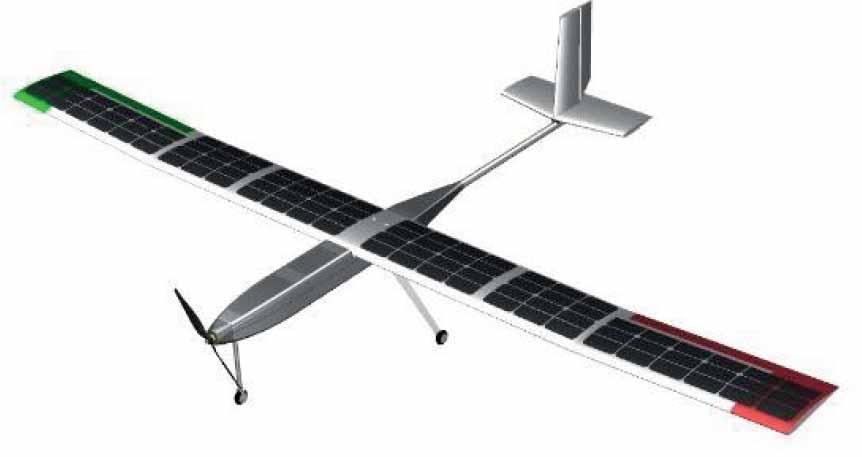
Visualization of the AZ-5 UAV research platform
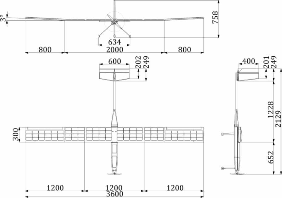
Basic dimensions of the AZ-5 UAV research platform
The development of the platform reached its final stage. The first version of the plane, named AZ-5A (configuration without photovoltaic installation), successfully completed the flight tests. The second prototype, AZ-5B (version with photovoltaic installation), is under development.
Nevertheless, developing new construction is a multidisciplinary process that demands considerable effort and coordination of diverse tasks. Therefore, the authors decided to support development works by a commercial RC plane as an intermediate test platform. Its designation is to perform avionics integration and verify its functionality in flight tests. A system for measuring and acquiring sun radiation intensity during flights has also been developed.
As a result, a set of unique flight parameters has been obtained. A different trajectory has been verified during flights, starting from manual flight and finishing on circular patterns with different radii.
Up to this time, particularly in recentyears, numerous trials have been conducted to develop small solar-powered UAVs. However, only a few prototypes realized the perpetual flight. A research team from Switzerland performed one of the most advanced research studies. Noth [1–3] successfully developed the Sky-Sailor aircraft. Oettershagen made essential contributions to the field of small solar-powered UAVs, which led to the development of AtlantikSolar [4,5]. In [6,7], he presented a set of flight data logs from perpetual flights. In [8], he validated the proposed solar power model. Dwivedi et al. published a series of papers [9–12] describing MARAAL aircraft. Dantsker etal. [13,14] developed Solar Flyer UAV and presented test results from long-endurance flights. Weider, with his team [15] developed SunSailor UAV. In Poland, there are only a few examples of research concentrated on this technology. Among them, the AGH Solar Plane [16] is notable.
To design the solar-powered aircraft correctly, the amount of solar radiation that can be collected must be precisely estimated. The UAV can perform complex maneuvers, and the solar cells can change the orientation with respect to the direction of the incoming radiation. Up to this time, several researchers have addressed the need to develop an accurate energy harvesting model for solar-powered UAVs [17–20]. Li et al. [21] presented a simulation that could predict the amount of collected solar energy and was partially validated by flight trials. Hrovatin and Žemva [22] presented and validated a model in a flight test using a small UAV named Bramor ppX. Rajendran and Smith [23] also proposed a model that can be used for predicting solar radiation and sizing UAVs. Morton and Papanikolopoulos [24], as well as Sineglazov and Kara-betsky [25], proposed a simple approach, suggesting that the captured solar power could be modeled using a sinusoid. However, the presented results were not validated against the experimental data in sufficient detail.
It is essential to note that creating reliable energy models for flying platforms requires considering several key phenomena. Such a model should be integrated, at the very least, with the kinematic description of motion. Often, the simple point mass models of the aircraft are adopted [26,27]. The geometry of the system must be taken into account. Zhang et al. [28] included each wing segment’s dihedral in the model’s bank angle. Ji et al. [29] investigated the mismatch loss problem in detail. Wu et al. [30] considered the equipping of a Z-shaped wing in solar cells. Most of the models are developed under the assumption of a clear sky [31]. For example, Huang et al. [32] reported the energy harvesting model and simulated the results for several cities in China, but again without experimental verification. However, neglecting clouds could significantly overestimate the total collected energy. For HALE aircraft, the reflected component could be neglected [33], but for small UAVs flying at low altitudes, this issue is not apparent. Gao et al. [34] suggested that for UAVs operating at very high altitudes, the influence of the roll and pitch angles on the amount of collected energy can be neglected. This assumption seems to be very rough. Martinez et al. [35] concluded that the roll angle can be ignored for predicting the amount of solar energy that UAVs can collect when the Sun is at high elevation, but not in the morning and evening (when the Sun is low above the horizon). Lee and Yu [36] considered the atmospheric transmittance. A detailed energy model for solar-powered UAVs was described by Wu et al. [37,38]. Brizon [39] presented a solar energy model for HALE platforms. He investigated the influence of several factors (latitude, longitude, and trajectory type) on the amount of collected energy. Meyer et al. [40] presented a simplified approach for predicting the amount of solar energy that UAVs can collect, but the method was not experimentally validated. Park et al. [41] developed a ground-based virtual flight system that mimics the real UAV’s dynamics and compared results with those from simulation.
The technology of LALE UAVs is not fully mature. Many of the aforementioned models were not sufficiently validated. To make the model realistic and practically usable, its parameters must be carefully tuned.
The primary contribution of this research is the description of solar radiation measurements evaluated in flight using a small UAV. The developed equipment is small, lightweight, and low-cost, making it suitable for adoption on other platforms. The aircraft and solar radiation models were developed and implemented in MATLAB/SIMULINK. These models were validated with the obtained data. The developed simulation might be used to design photovoltaic installations on solar-powered aircraft.
The structure of the paper is as follows. Chapter 2.1 describes the test platform. The solar radiation measurement system was presented in part 2.2. Section 2.3 shows mathematical models of the aircraft and solar radiation models. In part 2.4, the ground measurements of the power consumption were reported. Chapter 3 presents the results of the flight tests and model validation. The paper concludes with a summary of the main findings and their implications. Finally, further research directions are suggested.
The Multiplex Funcub NG RC airplane was used as a test platform (Fig. 3). The aircraft features a traditional design, characterized by a high-mounted wing, single engine, fixed landing gear, and a tailwheel configuration. It is characterized by ease of use and is frequently used as a training platform. The airplane has been modified in comparison to its original equipment.
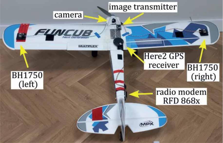
Test platform used in the experiments
Takeoff mass was m = 1,96 kg, wing area was Sw = 0,399 m2, span bw = 1,41 m, chord cw = 0,23 m, and overall length 1,050 m. Moments of inertia were obtained experimentally using a bifilar pendulum and are equal: Ixx = 0,07598 kg·m2, Iyy = 0,09504 kg·m2, Izz = 0,12134 kg·m2. The product of inertia Ixz = 0,00259 kg·m2 was calculated using the CAD model. The airplane’s standard equipment consists of a ROXXY BL C35-42-930 KV electric motor, a ROXXY BL Control 740S-BEC electronic speed controller, an APC 12x6E propeller, and a set of Hitec HS 55+ andHS 65HB servos. Power is provided by a single 3S package of 3200mAh capacity produced by Dualsky. The airplane is controlled using a Futaba T14SG radio controller and a Futaba R7008SB receiver module. Originally, the model weighed 1,380 kg with a wing loading of 3,46 kg/m2. Modifications have been performed to adapt the aircraft for test platform functionality. Additional equipment (equivalent to 42% of its initial weight) caused an increase in platform weight to 1,960 kg, resulting in a wing loading increase up to 5,66 kg/m2. Weight change is naturally connected with the reduction of maximum flight duration.
Among additional equipment, it is possible to distinguish the following hardware: the Cube Orange, Here2 GPS receiver, airspeed sensor, ultra-long range radio modem RFD 868x, FPV camera with vision transmitter AV TS832, 2 x Adafruit BH1750 light sensors, Arduino microcontroller with Datalogger Shield V1 equipped with RTC DS1307 and SD memory card slot, 9V backup battery for powering the Arduino and additional ballast needed to balance the test platform properly To reduce unpredictable platform behavior, it has been decided to disable the flaps operation.
The solar radiation measurement system was developed in cooperation with the School of Engineering and Built Environment (and Aviation) at Griffith University (in Brisbane, Australia).
Typically, the solar irradiance is measured using pyranometers or photovoltaic reference cells. However, such sensors are expensive and large, making it problematic to install them on small UAVs, such as Funcub. Due to this reason, it was necessary to develop a customized, relatively low-cost solution that could serve as an alternative to high-grade sensors.
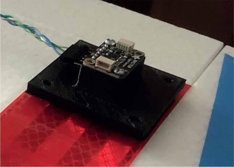
The system consists of the following components: two identical light sensors BH1750 (Fig. 4) located at the end of the wings (at the top surface), 3D printed sensor holders mounted with Velcro (Fig. 5), Arduino microcontroller, DataLogger shield V1.0 RTC DS1307 with SD card reader dedicated for Arduino, 32GB microSD card, 9V rechargeable lithium-ion battery and connection cables.

BH1750 light sensor
Sensor mounted on the surface of the left wing
The data recorder is based on the Arduino board (Fig. 6).
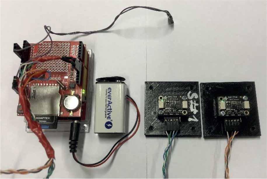
Completed set of solar radiation measurement system
The measurement system has been designed to be completely independent of autopilot hardware. To synchronize data registered by the autopilot and the developed system, a signal responsible for aileron deflection has been recorded to a microSD card.
Measurement system functionality has been obtained by programming the Arduino microcontroller using dedicated libraries. The data acquisition system communicates with light sensors and saves recorded information to the microSD card.
The first stage of the communication protocol checks was completed using two microcontrollers (Fig. 7).
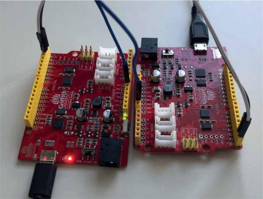
Microcontroller protocol communication test
Integration of the light sensor required setting individual IP addresses for each device. In further steps, a complete system was assembled on the stationary test bench (Fig. 8a).
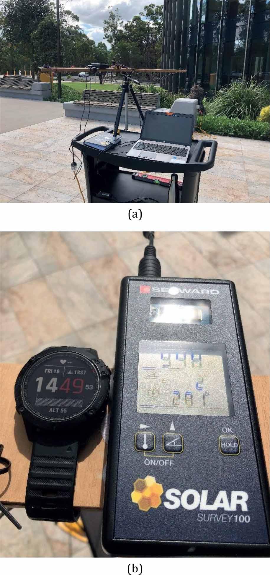
(a) Stationary test stand during experiments in Brisbane (b) Solar Survey 100 irradiance meter
The developed system estimates solar irradiance (a radiometric quantity) using information about illuminance (a photometric quantity).
The BH1750 light sensor outputs the illuminance (expressed in lux) directly. A set of preliminary measurements has been completed, providing that the sensor’s reading has been saturated at around 32000 lux. However, in outdoor conditions at noon, the illuminance can achieve more than 110000 lux. For this reason, it was necessary to modify the default setup and increase the sensor’s reading range to the required value. Improvements have been made with the change of device resolution, focusing on software code modification. Next, the procedure included a light sensor calibration from lux to power expressed as W/m2 delivered by the Sun to Earth’s surface, which was accomplished using the Solar Survey 100 irradiance meter (Fig. 8b). Finally, data were logged on the microSD at a frequency of 10 Hz. Additionally, the data stream was synchronized in time with the selected single reference signal from the autopilot (right aileron deflection angle). This allowed for the simultaneous analysis of the flight logs (from the autopilot) and the solar radiation measurement system.
The system successfully completed the stationary tests. It has been integrated with the RC airplane research platform in the next step. Sensors were mounted on the upper wing surface. The distance between devices is equal to 1,16 m. Additionally, the surfaces of both sensors were aligned with respect to each other. Minor mounting inaccuracies might influence the quality of the results. Nevertheless, this method was deemed sufficient for testing purposes. Because the airplane wing has a small inclination, it is expected to obtain slightly different readings from the light intensity sensor, as its vectors are not parallel.
Due to the fact that wires and sensor holders are located on the wing’s upper surface and are not integrated into the structure, the airplane’s aerodynamic characteristics may be slightly influenced, causing increased drag force.
A detailed mathematical model of the aircraft was developed to predict the amount of solar energy that can be collected during the flight.
It was assumed that the aircraft is a rigid body with 6 degrees of freedom. The coordinate systems used in the model are presented in Fig. 9. The navigation frame Onxnynzn is used to describe the position of the aircraft. Origin Ob of the body-fixed frame Obxbybzb is attached to the center of mass of the plane. Additionally, Ogxgygzg was used as the intermediate frame (axes of the Ogxgygzg are parrarel to Onxnynzn). Moreover, to define the aerodynamic properties wind frame Owxwywzw and wind-laboratory frame Owlxwlywlzwl were used.
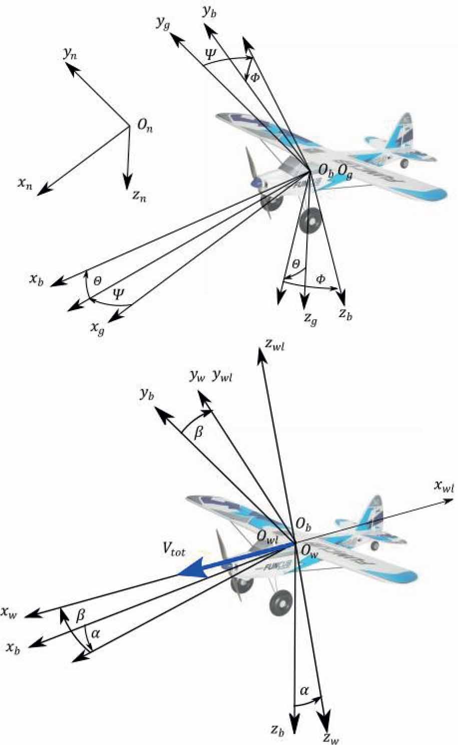
Coordinate systems used in the model
The equations of translational motion are as follows:
It was assumed that the aircraft possesses the vertical plane of symmetry, so Ixy = Izy = 0.
Quaternions were used to describe the altitude of the aircraft:
Velocity components in Onxnynzn are computed from the relation:
The gravity loads in body-fixed frame Obxbybzb frame were calculated as:
The torque generated by the gravity force is zero because the origin Ob of the Obxbybzb frame coincides with the center of mass of the plane.
The aerodynamic forces in the body-fixed frame are:
Additionally, δR – rudder deflection (positive trailing edge left).
The moment’s coefficients are:
The total speed is:
The aerodynamic characteristics of the plane were calculated using XFLR5 software. The coefficients (for undeflected control surfaces) are presented in Fig. 10.
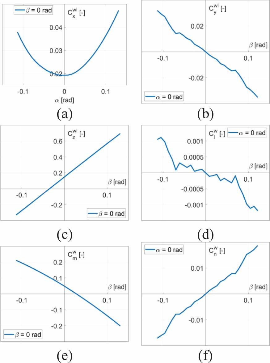
Aerodynamic coefficients of the airplane (a) drag (b) side force (c) lift force (d) rolling moment (e) pitching moment (f) yawing moment
Force coefficients are related in Owlxwlywlzwl frame, and moments (with respect to the center of mass) in Owlxwlywlzwl frame.
The stability and control derivatives of the Funcub plane are presented in Table 1.
Stability and control derivatives of the Funcub plane
| Longitudinal | Value | Unit | Lateral–directional | Value | Unit |
|---|---|---|---|---|---|
| 0,01920 | – | 0 | – | ||
| 0,01653 | 1/rad | –0,26240 | 1/rad | ||
| 1,53900 | 1/rad2 | –0,07607 | 1/rad | ||
| 0,29927 | 1/rad | 0,22320 | 1/rad | ||
| 0,00989 | 1/rad | 0 | 1/rad | ||
| 0,14840 | – | 0,11450 | 1/rad | ||
| 4,22000 | 1/rad | 0 | – | ||
| 7,08930 | 1/rad | –0,00789 | 1/rad | ||
| 0,49847 | 1/rad | –0,46079 | 1/rad | ||
| 0,03794 | – | 0,10362 | 1/rad | ||
| –1,68900 | 1/rad | –0,14324 | 1/rad | ||
| –9,69450 | 1/rad | 0,01302 | 1/rad | ||
| –1,20320 | 1/rad | 0 | – | ||
| 0,14330 | 1/rad | ||||
| –0,02406 | 1/rad | ||||
| –0,10615 | 1/rad | ||||
| 0 | 1/rad | ||||
| –0,05460 | 1/rad |
Data of the propeller were obtained from the dataset provided by the manufacturer (APC Propellers). The propulsive forces were calculated as:
The propeller thrust was calculated using the formula:
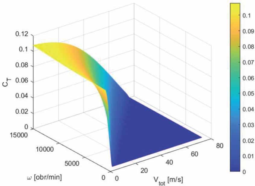
Thrust coefficient
The moments with respect to the aircraft center of mass were also taken into account:
The presented mathematical model of the aircraft was implemented in MATLAB/SIMULINK R2023a with Update 5. The equations of motion were integrated numerically using a 4th-order fixed-step solver (Runge-Kutta) with a time step size of 0,001 s.
The solar radiation model was developed to predict the amount of received solar radiation. The position of the Sun was parametrized using azimuth and elevation angles (Fig. 12) [23].
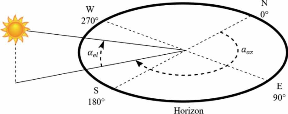
Solar azimuth and elevation angles
Solar declination was calculated as follows [46,47]:
Azimuth angle aaz was obtained from the relation [48]:
The inverse cosine trigonometric function returns values in the range from 0° to 180°. If the hour angle is negative, then aaz = 360°–aaz. In that way aaz falls in range from 0° to 360°.
The ASHRAE clear sky model was used to predict the amount of solar radiation received by the sensors. The changes in extraterrestrial radiation during the year are modeled as [46]:
The total irradiance is the sum of the beam, diffused, and reflected components [49,50]. The beam’s normal irradiance per unit area, (which is perpendicular to the sun rays) [46,51] was obtained as:
The diffuse horizontal irradiance per unit area on a horizontal surface [46,51]:
The coefficients τb and τd depend on the geographical location and vary during the year. Some tabulated values can be found, for example, in [46]. The coefficients b and d were obtained from the following relations [37,46,51]:
In Obxbybzb frame the unit vector along the zb axis (in the negative direction) have the following components
After several mathematical operations, the result is [51,52]:
When the cos λ is known, it can be used to calculate the amount of received power from the unit area [32, 51,53].
The sensors are installed only on the upper surface of the wing. If the surface of the sensor is oriented in the direction opposite to the Sun, then the direct component is [26,37,54]:
The diffuse irradiance is:
The solar radiation on the horizontal surface is:
For low attitude also, the reflected component was taken into account [55]:
The solar radiation model was implemented in MATLAB/SIMULINK and integrated with the numerical flight simulation of the aircraft (Fig. 13).
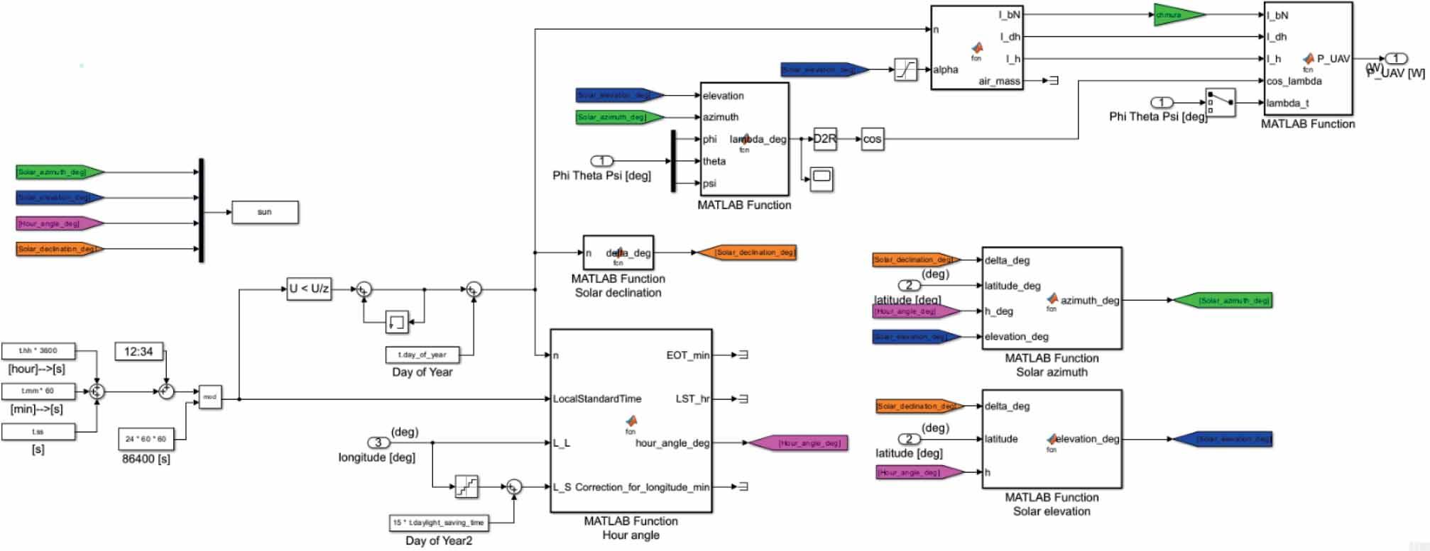
Solar radiation model implemented in SIMULINK
Moreover, the presented model of the Sun’s position was validated by comparing the results obtained from SIMULINK with those from the website https://www.suncalc.org. Next, the model was used to predict the amount of solar radiation and prepare the flight scenarios for the real experiments.
During research, it was required to estimate the power demand and energy consumption of the individual subsystems (electric engine, autopilot, telemetry, and sensors). The total energy consumption of the system is recorded in the flight logs. However, the power module used to monitor the battery state must be properly calibrated.
A series of ground tests was conducted to obtain the amount of power required by the components of the electric systems. Voltage and current were measured manually using a voltmeter (connected in parallel) and an ammeter (placed in series) between the main battery and autopilot.
It should be noted that a secondary power source powers the solar radiation measurement system. The obtained results are presented in Table 2.
Power consumption of system’s components
| Test case | Voltage [V] | Current [A] | Power [W] |
|---|---|---|---|
| Solar radiation measurement system | 9.11 | 0.075 | 0.683 |
| Avionics + propulsion (main motor off) | 12.40 | 0.575 | 7.130 |
| Avionics + propulsion (main motor on – at cruise RPM) | 9.55 | 29.460 | 281.343 |
| Avionics + propulsion (main motor on – maximum RPM) | 8.80 | 70.270 | 618.376 |
The energy consumption by the electronic components is practically constant. The power required by electronics is much smaller (below 3% of the total maximum value) than the power necessary to drive the electric motor. Increasing the angular speed of the motor results in a significant drop in the battery voltage.
A series of flight tests was conducted at different times of the day to collect the data. The experiments were evaluated at two locations: Zalesie (52,266874°, 20,751108°) and Przasnysz (53,009749°, 20,929911°) airfields (Fig. 14).
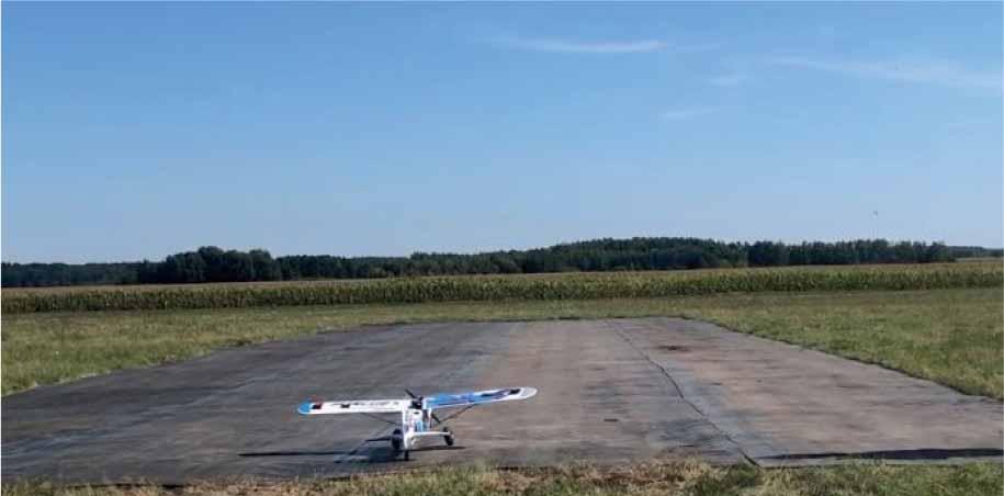
Aircraft ready to start at the runway in Przasnysz airfield.
The primary objectives of the experiments were to collect data on flight parameters and solar radiation, which are essential for validating the developed mathematical models.
The weather conditions were good, with low cloud coverage (in both locations). In Zalesie, the wind gusts’ maximum speed was no more than 3 m/s, but in Przasnysz, it was significantly higher (up to 6 m/s). The aircraft was controlled remotely by an experienced drone pilot. The experiments were realized in two flight modes: manual and semi-automatic. Additionally, the second operator observed the flight parameters (e.g., speed, altitude, battery state of charge) using the Ground Control Station. In that way, the aircraft ensured that it would correctly and safely complete the predefined mission scenario. The flight logs obtained from the autopilot were analyzed using Mission Planner software (https://ardupilot.org/planner/) and UAV Log Viewer (https://plot.ardupilot.org/#/).
Next, the developed models were validated using the obtained data. The input data to the model (geographic coordinates, date, and time of the trials) were set according to the measured data. The flight trials were documented with photographs, so it was possible to obtain the level of cloudiness. The flight logs were aligned in time with data from the solar radiation measurement system. In order to calculate the cross-correlation of two discrete-time signals (aileron deflection), the MATLAB function “xcorr” was used.
In the subsequent paragraphs, selected results from the experiments are presented.
This test was performed in Zalesie on 2023-09-08 (year-month-day). The data logging process started at 16:38:56 (HH:MM:SS, hours, minutes, and seconds) Central European Summer Time (CEST).
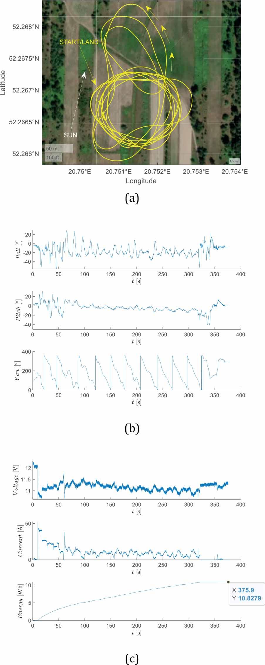
The aircraft took off at 16:45:54. In that case, the UAV was piloted only in manual mode. The aircraft flight path is presented in Fig.15a (data has been cropped to the time range of interest). As can be observed, the pilot has frequently repeated trajectories similar to airfield traffic patterns (in the counterclockwise direction when looking from the top). Small yellow arrows in Fig.15a mean the direction of motion. The white arrow indicates the solar azimuth (the direction of the sun’s rays). At the start, the solar azimuth was 249,57° and the elevation was 22,04°. Azimuth is measured from North in a clockwise direction, and elevation from the horizontal plane (please see the convention in Fig.12). The roll, pitch, and yaw angles are presented in Fig.15b. In Fig.15c, the battery voltage, current, and the total amount of energy consumed by the aircraft are shown.
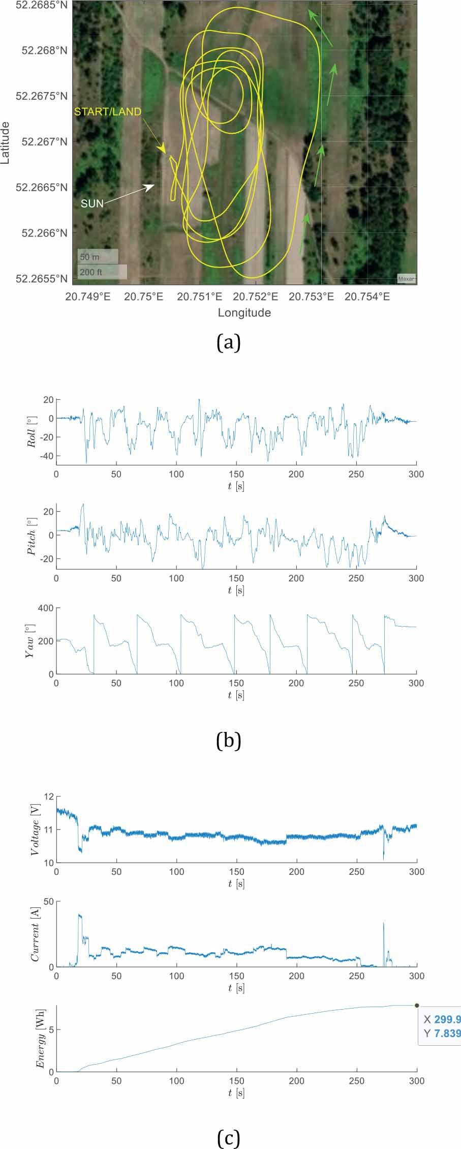
Aircraft flight parameters (a) position (b) roll, pitch, yaw angles (c) battery voltage, current, and consumed energy (case 1)
The measured roll angle was between -48,16° and +20,74° (the plot is asymmetrical because the aircraft performed left turns). From the yaw angle plot, it can be concluded that approximately 8 full loops were evaluated in flight.
The voltage decreases slowly with time. The current has the highest amplitude at the beginning of the mission because then the aircraft performs the start and the ascending flight. To realize the mission 7.84 Wh of energy was spent.
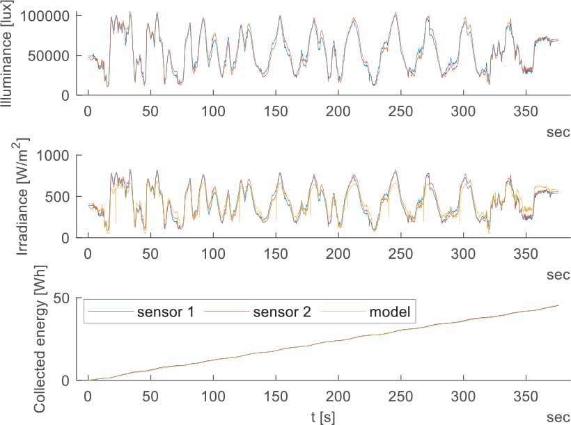
In Fig.16, the measured solar illuminance is presented. The measured solar illuminance was converted into solar radiation intensity using calibration coefficients that were obtained experimentally. Then, the obtained results were integrated in time to estimate the energy that could be collected (per 1 square meter).
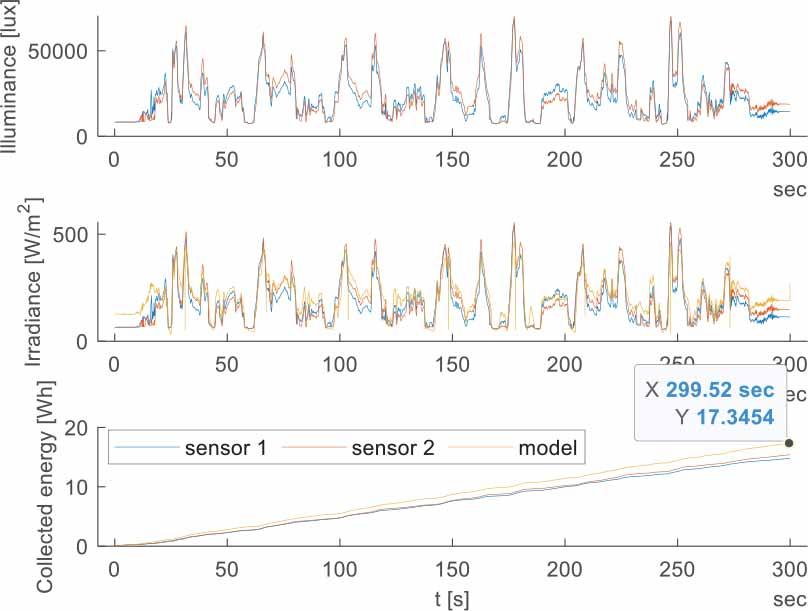
Solar illuminance, radiation intensity, and energy (case 1)
The maximum possible amount of solar radiation intensity is approximately 554,6 W/m2. The amplitude varies significantly due to changes in altitude. The radiation received by sensors strongly correlates with the roll and pitch angles. The aircraft performed a set of maneuvers. The intensity depends strongly on the angle between the incoming ray and the sensor’s surface.
Moreover, it can be observed that the data from both sensors differ a bit. The main reason for that phenomenon is the wing’s dihedral angle and the sensors’ minor mounting imperfections.
The amount of energy increases monotonically with time. The data from sensor 1 indicate that collecting 14.78 Wh of energy (from 1 square meter) is possible in these conditions. Using data from sensor 2, it was found that this result is slightly higher, 15.41 Wh.
The experimental radiation intensity values are in close agreement with the model predictions. The model overestimated the amount of collected energy (17,35 Wh).
The typical overall efficiency of photovoltaic systems that are used on solar-powered UAVs is around 20% [7]. This means that theoretically, the 2.956 Wh of energy can be obtained (using sensor 1 data).
The Multiplex Funcub NG is unable to achieve perpetual flight using only solar energy because the energy required for propulsion is significantly higher than the amount of energy that can be harvested from solar radiation.
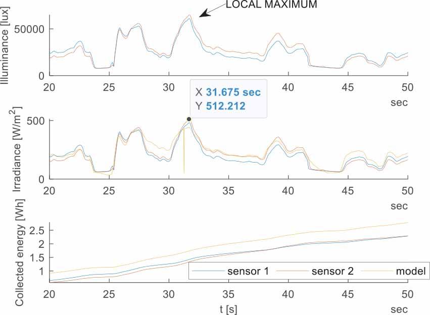
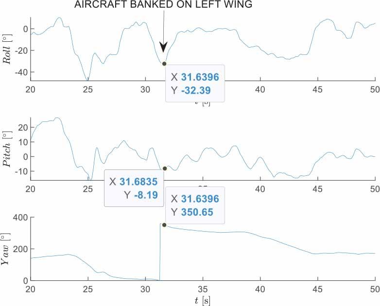
It is worthwhile to take a closer look at the results to understand the relationship between the Euler angles and the amount of solar radiation received. The selected data portion (from 20 s to 50 s) is shown in Fig. 17 and Fig. 18 to make the details more visible.
Roll, pitch, yaw angles (case 1, enlarged view)
Solar illuminance, radiation intensity, and energy (case 1, enlarged view)
One of the peaks of the solar radiation occurred approximately at time 31.6 s (please see the datatip in Fig. 17). Then, the aircraft was banked on the leftwing (roll angle is negative and equal to around –32°) and moved at the yaw angle of 350° (from South to North). That means the solar radiation sensors were pointed in the direction of the oncoming radiation. The sketch of the aircraft location on the analyzed portion of the flight path is presented in Fig. 19.
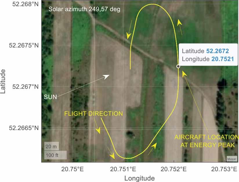
Approximate aircraft location at energy peak (case 1, enlarged view)
On the other hand, in 50 s, the amount of received solar radiation is relatively small because the aircraft moved from North to South, and the roll angle is ≈4.5° (the sensors were not pointed directly to the Sun).
Scenario 2 was also completed in Zalesie on 2023-09-12. The data logging in autopilot was initiated at 13:07:02 CEST. The plane took off at 13:14:42. In this experiment, the aircraft was piloted in both manual and semi-automatic modes. The resulting flight path is presented in Fig. 20a. The plane moved in a counterclockwise direction. The solar position (azimuth and elevation) was 193,19° and 41,23°, respectively.
Aircraft flight parameters (a) position (b) roll, pitch, yaw angles (c) battery voltage, current, and consumed energy (case 2)
The roll angle (Fig. 20b) was in the range from – 56,25° to +29,17°. Also, the pitch angle was between –41.31° to +31.09°. The yaw angle indicates that the aircraft realized more than 11 loops.
The current (Fig. 20c) drops rapidly after 320 s because the plane landed and then was taxiing on the runway. The aircraft spent 10,83 Wh of energy during the mission.
In Fig. 21, the solar radiation measured in the second flight trial is shown.
Solar illuminance, radiation intensity, and energy (case 2)
The solar radiation intensity exhibits a sinusoidal pattern corresponding to changes in the orientation angles. The maximum value of solar radiation intensity is 829,3 W/m2 (significantly higher than in case 1). From sensor 1, it was estimated that collecting 45,21 Wh of solar energy is possible (per 1 square meter). Using sensor 2, this value was estimated to be 45,26 Wh.
The model predicted that the amount of energy that can be harvested is 45,65 Wh, which is close to the real values.
Again, assuming the aircraft can be equipped with solar panels (1 square meter in area) and the energy can be harvested with an efficiency of 20%, the obtained value is 9,042 Wh.
In this case, the amount of harvested energy is still insufficient to cover the instantaneous energy demand. Moreover, from a practical point of view, the hypothetical system cannot accumulate energy for the onboard batteries (because the energy consumption of 10,83 Wh was higher than production). As a matter of fact, it would not be possible to achieve perpetual flight functionality over a longer period.
In Fig. 22 and Fig. 23, the selected data portion (from 220 s to 260 s) is shown in an enlarged view.
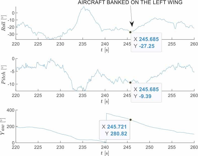
Roll, pitch, yaw angles (case 2, enlarged view)
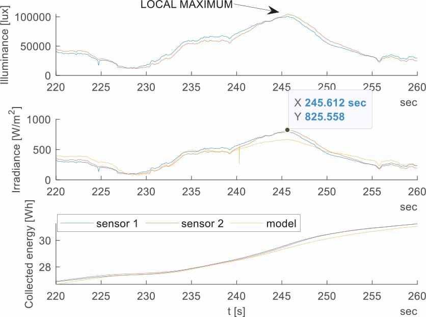
Solar illuminance, radiation intensity, and energy (case 2, enlarged view)
One of the energy peaks occurred at time 245,6 s. The aircraft performed a left turn and was banked on the leftwing (roll angle is –27,25°, please see Fig. 22). This means the solar radiation sensors were pointed toward the incoming sunlight. The situation scheme with the selected portion of the flight path is presented in Fig. 24.
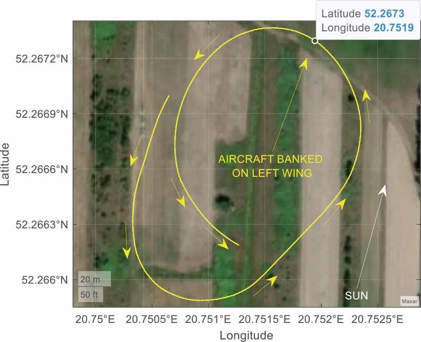
Approximate aircraft location at energy peak (case 2, enlarged view)
In case number 3, the experiment took place in Przasnysz on 2023-09-21. The data logging system was initiated at 15:41:26, and the plane taxied for a while. Next, the aircraft took off at 15:45:17. The plane started and landed in manual mode, but most of the mission was realized in loiter mode. The radius of the circular trajectory (Fig. 25a) was larger when compared to case 2. Solar azimuth and elevation angles were 234,53° and 24,41°.
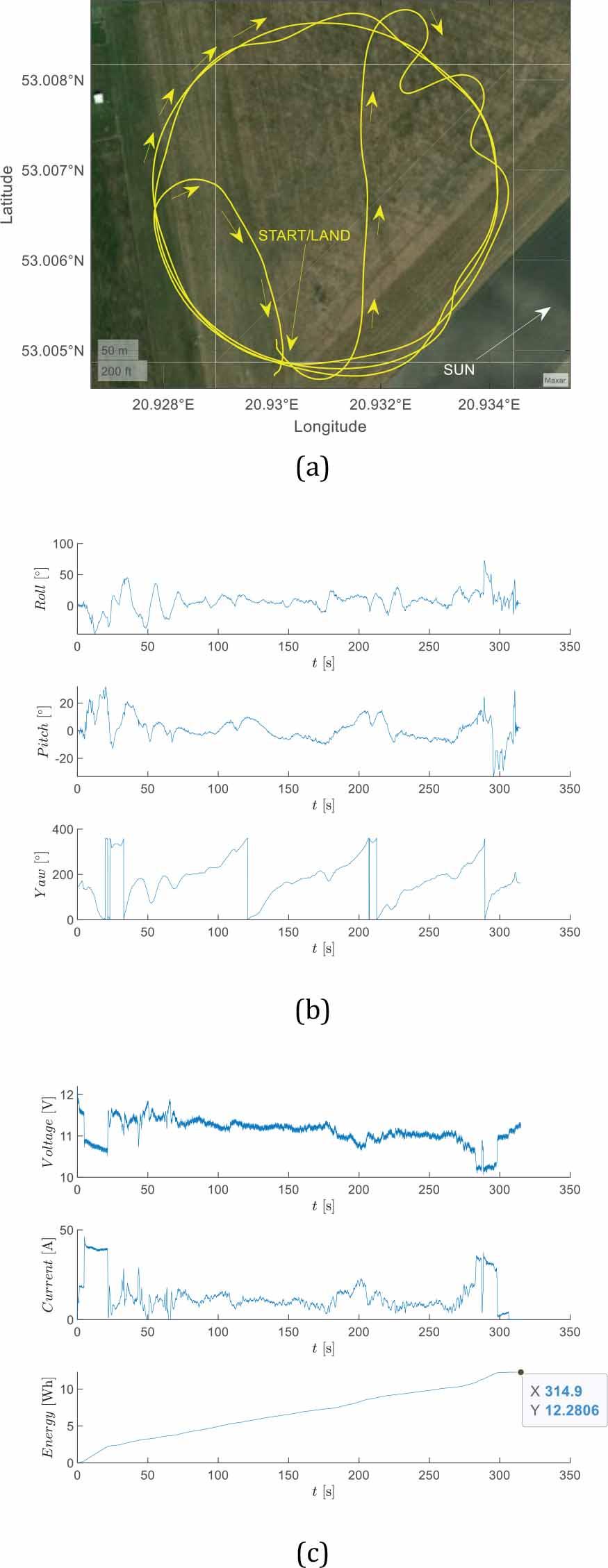
Aircraft flight parameters (a) position (b) roll, pitch, yaw angles (c) battery voltage, current, and consumed energy (case 3)
The roll angle (Fig. 25b) varied significantly from –45,75° up to 73,12°. To fulfill the mission, 12,28 Wh of the energy was spent by the onboard electronic system (Fig. 25c).
The light radiation intensity is presented in Fig. 26.
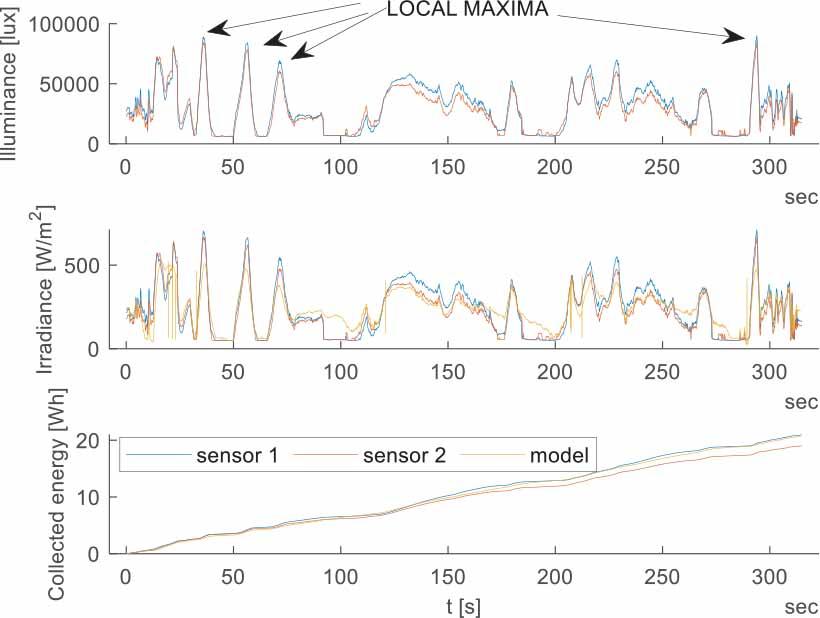
Solar illuminance, radiation intensity, and energy (case 3)
The maximum measured value of the radiation intensity is 701,6 W/m2.
Using data from sensor 1, it was calculated that 20,93 Wh of energy can be collected (from 1 square meter of surface). Data from sensor 2 indicates a bit lower value of 19,01 Wh. The model predictions (20,72 Wh) are between the values from both sensors.
The enlarged view of the selected data portion is shown in Fig. 27 and Fig. 28.
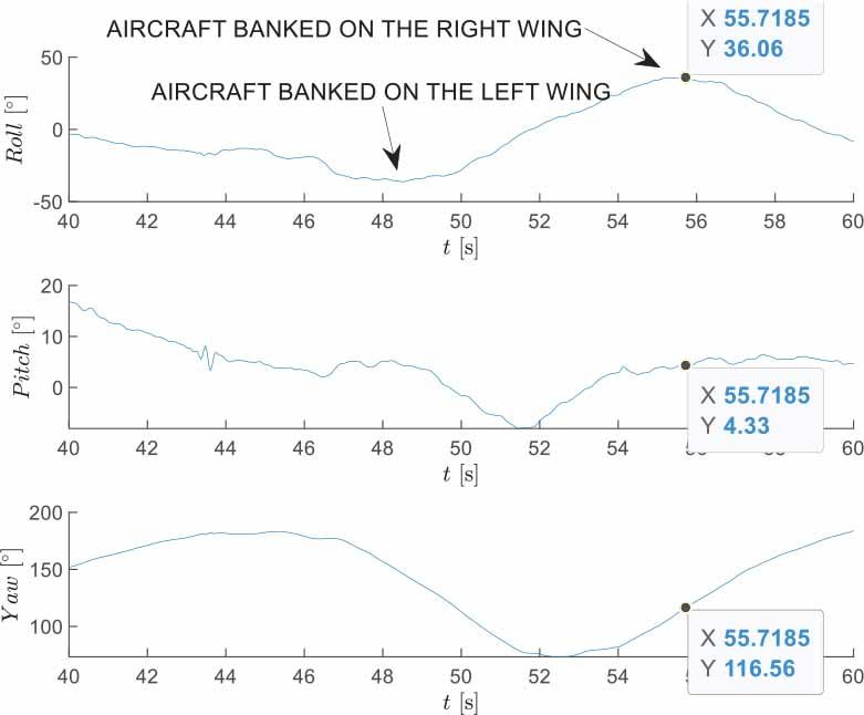
Roll, pitch, yaw angles (case 3, enlarged view)
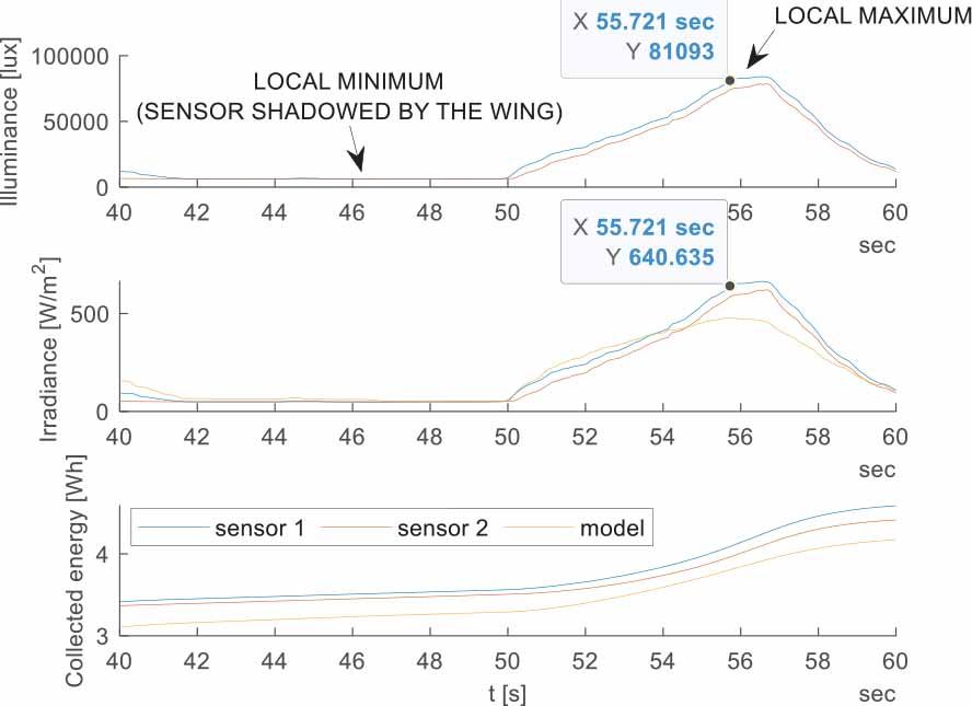
Solar illuminance, radiation intensity, and energy (case 3, enlarged view)
For the selected part of the trajectory, the aircraft performed two rapid turns (please see Fig. 29). In the first turn, it was banked to the left, and as a result, the wing shaded the solar radiation sensors. Between 40 s and 50 s, the irradiance was smaller than 60 W/m2 (the curve is practically flat for this time range). In the second turn, the aircraft banked on the right wing. The maximum roll angle occurred at 55.7 s and is equal to 36,06°.
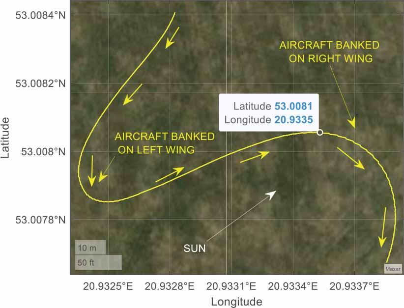
Approximate aircraft location at energy peak (case 3, enlarged view)
As a result, the sensors were pointed directly at the Sun. In Fig. 28, at 55,7 s, the local maximum of the signal was observed.
This paper presents the methodology for inflight solar radiation measurements using a small unmanned aerial vehicle.
Among the main goals of the conducted research, the following stages can be distinguished: avionics system integration and testing, flight experiments, data acquisition from the flight and solar systems, analysis of recorded data, and performance of computer simulations based on the obtained results. Completed works are the intermediate stage of developing the primary research platform – the AZ-5 solar UAV – and can be directly implemented based on the gained experience.
To adapt the RC airplane for research platform requirements, a set of modifications has been made. Among them, it is possible to distinguish the solar radiation measurement system and additional avionics integration. The undeniable drawback of the modifications is an increase in platform weight, and therefore, a reduction in its total flight time.
Experience from the development of the solar radiation measurement system, e.g., hardware programming and conducted functionality tests, proved that its subcomponents should be selected with particular care. Sensor quality, including sampling frequency and accuracy, is a key factor influencing the final results. Another significant aspect is light sensor calibration, which allows for direct conversion from lux to W/m2. It is essential to note that the proposed measurement device has lower accuracy than high-performance grade irradiance meters. However, it allows for the collection of quantitative data at a reasonable cost.
The next research goal was to validate a solar radiation model. From recorded flight data obtained at two locations in Poland and at different times of day, a representative dataset consisting of 3 flights has been selected. All flights have been performed in good weather conditions, with small to moderate cloud coverage and wind gusts of less than 3 m/s in Zalesie and up to 6 m/s in Przasnysz. Flight conditions have been incorporated into the simulation model, including airplane orientation angles, exact time (date, hour, and minute), flight duration, and geographical location. As a result, an irradiance function was obtained.
A comparison of simulation data with recorded data demonstrated the high quality of the mathematical model and its accuracy at a level of around 90% or above.
Moreover, some results may be initially confusing and not meet the above requirement. Namely, as can be observed from the radiation intensity figures, there are regions where the simulation model differs from the recorded values by more than 10%. This phenomenon is observed when an airplane flies below 25 m above ground level or remains on the ground in Zalesie. It is caused by the fact that the research platform was placed in the shadows cast by local objects (tall trees), and direct sun radiation components did not contribute to the solar radiation measurement. In fact, the developed solar radiation simulation model is assumed to be a valuable simulation device capable of reflecting actual flight conditions.
Lastly, an assessment of the modified Multiplex Funcub NG research platform’s capability to perform perpetual solar flights is also considered. Analysis of battery voltage, current, and energy consumption, as well as solar illuminance and estimated irradiance, yields several conclusions. The average power required during the performed flight tests varies from approximately 77 W to 142 W, depending on the flight mode selection and wind conditions. Flights performed in automatic mode with small wind gusts provide the lowest energy consumption. Flying with strong winds causes the highest energy usage.
During completed tests, the average possible power production from the hypothetical photovoltaic system varies from 17.6 W to 35 W, assuming an overall efficiency of 20% and complete coverage of the wing’s upper surface (0,399 m2for Funcub NG). A battery capacity of 35.52 Wh would not allow for accumulating enough energy to continue flights during lower Sun positions above the horizon (morning and evening hours).
The above analysis clearly states that the intermediate research platform Funcub NG cannot achieve perpetual solar flights because it requires a significant amount of energy. The data obtained will be used to design and develop the photovoltaic installation of the AZ-5 solar-powered aircraft. This aircraft (in contrast to Funcub NG) was specially designed and had much lower energy consumption and a high lift- to-drag ratio.