

Feedback linearization is a widely-used control technique for aerodynamic systems. This method linearizes non-linear systems globally, which provides a linear closed-loop system for controlling aerodynamic systems. Feedback linearization has been shown to be effective in controlling aerodynamic systems, even in the presence of non-linearities and cross-couplings. Its popularity in the field of control engineering can be attributed to its reliability and ease of implementation. Recent research has continued to demonstrate the effectiveness of feedback linearization for controlling aerodynamic systems. For example, in a study by Kim et al. [1], feedback linearization was applied to a helicopter model to improve its control performance. The results showed that the feedback-linearization approach effectively reduced steady-state error and improved the transient response of the system. In another study by Li [2], feedback linearization was used to control a flapping-wing aircraft. In [3, 4], there are presentations of the results of controlling aerodynamic autonomous systems such as quad-rotors and helicopters.
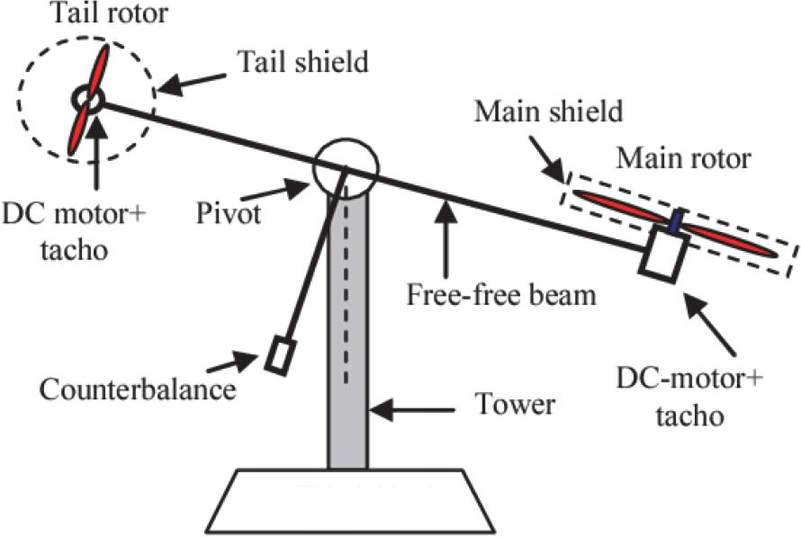
The Twin Rotor MIMO System (TRMS) is a wellestablished benchmark for flight control experiments and the validation of control theories. This system simulates the dynamics of a helicopter, with two inputs and two outputs that are cross-coupled. The TRMS provides a challenging platform for testing control techniques due to its non-linearities and complexity. Its close correlation to real flight dynamics makes it an ideal system for evaluating the performance of control systems under challenging conditions. Its use as a benchmark system has been widely recognized in the control engineering community.
A number of recent studies on the TRMS have also focused on improving its control performance [5–7], using to validate the accuracy of important non-linear and hybrid control techniques such as backstepping, adaptive feedback linearization, and robust control. For instance, in a study by Wang and colleagues [8], a hybrid control method was applied to the TRMS to achieve improved regulation and trajectory tracking. Another study by Zhang et al. [9] applied a model predictive control (MPC) approach to the TRMS, with the aim of improving its regulation and tracking performance.
The present work makes a significant contribution to the field of feedback linearization and the control of aerodynamic systems. By combining the feedback linearization control theory with the Thau observer, we were able to achieve better control performance than in previous studies. The use of the twin-rotor MIMO system as a benchmark allowed us to validate the effectiveness of our control approach in a real-world scenario. The simulation and real-time experiments conducted in this work showed promising results in both regulation and trajectory-tracking tasks, demonstrating the potential of this control approach in practical applications.
This proposed new method can be used to control robot systems in general Using this approach to control real helicopters may be possible, taking into consideration the helicopter system’s specifications.
The remainder of this paper is organized as follows. Section 2 presents the mathematical model of the twin-rotor MIMO system. Section 3 focuses on the feedback linearization control theory and its mathematical proof of stability in the closed-loop system, including the system, controller, and observer. The results of both the simulation and real-time experiments are presented and discussed in Section 4. Finally, in Section 5, we provide conclusions and future work suggestions to further advance our findings. Throughout the paper, we illustrate and analyze the results to aid in a comprehensive understanding of our work.
Twin Rotor MIMO System (TRMS)
In this sub-section we will present the TRMS model, we will follow a physical modelling using the laws of aerodynamics, mechanics and electricity to have a non-linear model.
- -
As it is a being a nonlinear and multi-variable system; the dynamics of the TRMS can be translated through equations describing the moments of force and inertia.
- -
The mathematical model is developed by making some simplifications; we suppose that:
- -
Motor dynamics can be described by firstorder differential equations as a function of the joint variables of the mechanism and vice-versa.
- -
The friction in the system is of the viscous type.
- -
Rotation can be described in principle as the movement of a pendulum.
- -
These are simplifying assumptions, they are made to simplify the modelling, these three assumptions presented above are argued, by the fact of the chosen operating range, as well as which slow operating mode chosen, without forgetting the mechanical structure of the system that allows us to make the 3rd hypothesis.
Modeling of the plant used here follows the same method as our precedent works [11, 21]; after rearrangement of equations of moments and forces we can get the following non-linear state representation:
We have the state vector:
Where ψ and φ are the pitch and yaw angle respectively.
τ1 and τ2 are the torques of the two motors of pitch and yaw respectively.
This system is in the form
Where
The TRMS parameters – from the “feedback” manufacturer
| Parameters | Values |
|---|---|
| I1 – main rotor moment of inertia | 6.8.10-2 Kg/m2 |
| I2 – tail rotor moment of inertia | 2.10-2 Kg/m2 |
| a1 – nonlinearity parameters | 0.0135 |
| b1-nonlinearity parameters | 0.0924 |
| a2-nonlinearity parameters | 0.02 |
| b2-nonlinearity parameters | 0.09 |
| Mg-moment of gravity | 0.32 N.m |
| B1ψ – parameter of the friction moment function | 6.10-3 N.m.s/rad |
| B2ψ – parameter of the friction moment function | 1.10-3 N.m.s/rad |
| B1ϕ – parameter of the friction moment function | 1.10-1N.m.s/rad |
| B2ϕ – parameter of the friction moment function | 1.10-2 N.m.s/rad |
| Kgy – gyroscopic moment parameter | 0.5 S/rad |
| K1-gain of motor 1 | 1.1 |
| K2gain of motor 2 | 0.8 |
| T11 – motor 1 denominator parameter | 1.1 |
| T10 – motor 1 denominator parameter | 1 |
| T21 – motor 2 denominator parameter | 1 |
| T20 – motor 2 denominator parameter | 1 |
| Tp – coupling moment parameter | 2 |
| To – coupling moment parameter | 3.5 |
| Kc–-coupling moment gain | -0.2 |
The exact linearization of nonlinear systems constitutes a natural and promising method, making it possible to obtain a linear input-output behavior by implement a loop. Subsequently, the whole linear theory can be applied [10–12]. Advanced control methods often include several loops including a feedback linearization. Input-output linearization plays an important role in a field like robotics, where the calculated torque method is a special case of input-output linearization [13].
Consider the following nonlinear system in affine form as input:
With x ∈ ℝn; u ∈ ℝm and y ∈ ℝp as the state vector, input and outputs of the system, respectively.
f(x), g(x) and h(x) are sufficiently regular functions in a domain D ⊂ ℝn Applications f:D → ℝn and g: D → ℝn call the vector fields in the domain D; and the application h:D → ℝn is the output immersion.
The solution for SISO systems can be easily generalized to multivariate systems. We then obtain the sufficient condition given by [11].
Given the system in the form of (1), we try to find, if possible, a regular static state looping, such as
With β(x) inversible, such as, for all i = 1….. p, given:
Let
The solution to this problem is given by a result similar to [11]; however, the condition here becomes necessary and sufficient.
Let (ρ1,…,ρp) be the set of infinite zeros per row of the system. Remember that these are defined as follows:
Recall that ρi, corresponds to the first derivative of yi, which explicitly shows the control law u:
With the multiplicative term of u designating the concatenation of the terms
Let Δ(x) be the matrix defined by:
This matrix is called the system decoupling matrix.
This condition on Δ(x) being satisfied — the state feedback defined by equation (2) — decouples the system ∑, such that:
Moreover, the looped system has a linear input output behavior described by:
The linear system obtained by this mathematical transformation is a chain of integrators with ρi poles at the origin; it is therefore unstable, hence the need for a stabilizing control that guarantees a certain level of performance for the system according to a specification. Loads [13]. In this paper we have contented ourselves with a placement of poles by linear state feedback.This can also be a dynamic output feedback, which uses the states of the physical system estimated by the Thau observer.
The results obtained by Thau were generalized by Kou et al. [15] and Banks [16]. This method does not constitute a systematic technique for the synthesis of an observer, but rather gives a sufficient condition of the exponential stability of the observation error [14].
Let us consider the nonlinear system, which can be put into the following form:
Where x(t) ∈ ℜn represents the state of the system,
f(x) : ℜn → ℜn is a differentiable vector field.
u(t) ∈ ℜm is the control vector.
y(t) ∈ ℜp is the output vector.
Thus, the system
The lemma in [18] characterizes the exponential convergence of this observer.
Given the following nonlinear TRMS model (shown in the 2nd section):
The state and output vectors are given by:
- -
Centralized architecture
We start with the successive derivations of the first output ψ, which makes the term of the commands appear in its third derivative,This allows us to know its relative degree, ρi = 3. The expressions containing the sign functions are not differentiable, so that they will be considered disturbances and omitted from the nonlinear model for the synthesis of the linearization feedback. The synthesis model is given by Either
\psi = {x_1};\dot \psi = {x_2};\varphi = {x_3};\dot \varphi = {x_4};{\tau _1} = {x_5}; \matrix{ {{f_1}(x) = {x_2}} \hfill \cr {{f_2}(x) = {{{a_1}} \over {{I_1}}}x_5^2 + {{{b_1}} \over {{I_1}}}{x_5} - {M_g}\sin \left( {{x_1}} \right) - {{{B_{1\psi }}} \over {{I_1}}}{x_2} - {{{k_{gy}}} \over {{I_1}}}\cos \left( {{x_1}} \right){x_4}\left( {{a_1}x_5^2 + {b_1}{x_5}} \right)} \hfill \cr {{f_3}(x) = {x_4}} \hfill \cr {{f_4}(x) = {{{a_2}} \over {{I_2}}}x_6^2 + {{{b_2}} \over {{I_2}}}{x_6} - {{{B_{1\varphi }}} \over {{I_2}}}{x_2} - {{{k_c}} \over {{I_2}}}1.75\left( {{a_1}x_5^2 + {b_1}{x_5}} \right)} \hfill \cr {{f_5}(x) = {{{T_{10}}} \over {{T_{11}}}}{x_5}} \hfill \cr {{f_6}(x) = {{{T_{20}}} \over {{T_{21}}}}{x_6}} \hfill \cr {f(x) = {{\left[ {{f_1}(x){f_2}(x){f_3}(x){f_4}(x){f_5}(x){f_6}(x)} \right]}^T}} \hfill \cr {g(x) = G = \left[ {\matrix{ 0 & 0 & 0 & 0 & {{{{k_1}} \over {{T_{11}}}}} & 0 \cr 0 & 0 & 0 & 0 & 0 & {{{{k_2}} \over {{T_{12}}}}} \cr } } \right]et h{\rm{(}}x{\rm{)}}} \hfill \cr { = \left( \matrix{ {x_1} \cr {x_3} \cr} \right)} \hfill \cr } Calculation of the successive Lie derivatives yield:
11 \left\{ {\matrix{ {{L_f}h(x) = {{\partial h(x)} \over {\partial x}}f(x)} \cr {\left[ {\matrix{ 1 \hfill & 0 \hfill & 0 \hfill & 0 \hfill & 0 \hfill & 0 \hfill \cr 0 \hfill & 0 \hfill & 1 \hfill & 0 \hfill & 0 \hfill & 0 \hfill \cr } } \right]f(x)} \cr { = \left[ \matrix{ {f_1}(x) \hfill \cr {f_3}(x) \hfill \cr} \right] = \left[ \matrix{ {x_2} \hfill \cr {x_4} \hfill \cr} \right]} \cr {L_f^2h(x) = {{\partial \left[ {{L_f}h(x)} \right]} \over {\partial x}}f(x)} \cr {\left[ {\matrix{ 0 \hfill & 1 \hfill & 0 \hfill & 0 \hfill & 0 \hfill & 0 \hfill \cr 0 \hfill & 0 \hfill & 0 \hfill & 1 \hfill & 0 \hfill & 0 \hfill \cr } } \right]f(x)} \cr { = \left[ \matrix{ {f_2}(x) \hfill \cr {f_4}(x) \hfill \cr} \right]} \cr {L_f^3h(x) = {{\partial \left[ {L_f^2h(x)} \right]} \over {\partial x}}f(x)} \cr } } \right. 12 L_f^3h(x)\left[ {\matrix{ {{{{k_{gy}}} \over {{I_1}}}\sin \left( {{x_1}} \right){x_4}\left( {{a_1}x_5^2 + {b_1}{x_5}} \right)} & { - {{{B_{1\psi }}} \over {{I_1}}}} \cr { - {M_g}\cos \left( {{x_1}} \right){x_2}} & 0 \cr 0 & { - {{{k_{gy}}} \over {{I_1}}}\cos \left( {{x_1}} \right)} \cr \ldots & {\left( {{a_1}x_5^2 + {b_1}{x_5}} \right)} \cr \ldots & {{{{B_{1\varphi }}} \over {{I_2}}}} \cr } \matrix{ 0 & \cdots \cr 0 & \cdots \cr {{{{b_1}} \over {{I_1}}} - {{{k_{gy}}} \over {{I_1}}}\cos \left( {{x_1}} \right)} & 0 \cr {{x_4}\left( {2{a_1}{x_5} + {b_1}} \right)} & {} \cr { - {{{k_c}} \over {{I_1}}}1.75\left( {2{a_1}{x_5} + {b_1}} \right)} & {{{2{a_2}} \over {{I_2}}}{x_6} - {{{b_2}} \over {{I_2}}}} \cr } } \right]f(x) 13 {_0}(x) = L_f^3h(x) = \left[ {\matrix{ {{{{k_{gy}}} \over {{I_1}}}\sin \left( {{x_1}} \right){x_4}{x_2}\left( {{a_1}x_5^2 + {b_1}{x_5}} \right) - {M_g}\cos \left( {{x_1}} \right){x_2}} & 0 \cr { - {{{B_{1\psi }}} \over {{I_1}}}{f_2}(x)} & 0 \cr 0 & 0 \cr { - {{{k_{gy}}} \over {{I_1}}}\cos \left( {{x_1}} \right)\left( {{a_1}x_5^2 + {b_1}{x_5}} \right){f_4}(x)} & {{{{B_{1\varphi }}} \over {{I_2}}}{f_4}(x)} \cr {{{{T_{10}}{k_{gy}}} \over {{T_{11}}{I_1}}}cos\left( {{x_1}} \right){x_4}{x_5}\left( {2{a_1}{x_5} + {b_1}} \right) - {{{T_{10}}{b_1}} \over {{T_{11}}{I_1}}}{x_5}} & {{{{T_{10}}{k_c}} \over {{T_{11}}{I_2}}}1.75\left( {{a_1}x_5^2 + {b_1}{x_5}} \right)} \cr 0 & { - {{2{a_2}} \over {{I_2}}}{{{T_{20}}} \over {{T_{21}}}}x_6^2 - {{{T_{20}}{b_2}} \over {{T_{21}}{I_2}}}{x_6}} \cr } } \right] 14 {L_g}L_f^2h(x) = {{\partial \left[ {L_f^2h(x)} \right]} \over {\partial x}}G 15 \matrix{ {{L_g}L_f^2h(x) = \left[ {\matrix{ {{{{k_{gy}}} \over {{I_1}}}\sin \left( {{x_1}} \right){x_4}\left( {{a_1}x_5^2 + {b_1}{x_5}} \right) - {M_g}\cos \left( {{x_1}} \right){x_2}} \cr 0 \cr \cdots \cr \cdots \cr } } \right.} \cr {\matrix{ { - {{{B_1}\psi } \over {{I_1}}}} \cr 0 \cr { - {{{k_{gy}}} \over {{I_1}}}\cos \left( {{x_1}} \right)\left( {{a_1}x_5^2 + {b_1}{x_5}} \right)} \cr {{{{B_{1\varphi }}} \over {{I_2}}}} \cr } } \cr {\left. {\matrix{ 0 & \cdots \cr 0 & \cdots \cr {{{{b_1}} \over {{I_1}}} - {{{k_{gy}}} \over {{I_1}}}\cos \left( {{x_1}} \right){x_4}\left( {2{a_1}{x_5} + {b_1}} \right)} & 0 \cr { - {{{k_c}} \over {{I_1}}}1.75\left( {2{a_1}{x_5} + {b_1}} \right)} & {{{2{a_2}} \over {{I_2}}}{x_6} - {{{b_2}} \over {{I_2}}}} \cr } } \right]G} \cr } 16 \Delta (x) = {L_g}L_f^2h(x) = \left[ {\matrix{ {{{{k_1}{b_1}} \over {{T_{11}}{I_1}}}} & 0 \cr { - {{{k_1}{k_{gy}}} \over {{T_{11}}{I_1}}}} & {} \cr {\cos \left( {{x_1}} \right){x_4}\left( {2{a_1}{x_5} + {b_1}} \right)} & {} \cr { - {{{k_1}{k_c}} \over {{T_{11}}{I_2}}}1.75\left( {2{a_1}{x_5} + {b_1}} \right)} & {{{{k_2}} \over {{T_{21}}}}\left( {{{2{a_2}} \over {{I_2}}}{x_6} - {{{b_2}} \over {{I_2}}}} \right)} \cr } } \right]
One can easily verify that the determinant of Δ(x) is different from 0:
With the condition that the sum of the relative degrees of the two outputs of the system equal to n = 6 (the order of the system), the control de?ined by the equation (2), and (8) globally linearizing and fully decoupling the TRMS system (no dynamic zeros).
The linear system thus obtained is in the form of two decoupled triple integrators, described by:
With implemented control as:
To stabilize for the desired performance, linearized state feedback by input-output linearization under the state delivered by the Thau observer with integral action will be applied to the auxiliary command inputs.
- 1)
Linearized state feedback
19 \left\{ {\matrix{ {{v_1} = {k_{11}}{y_{c1}} - {k_{11}}{z_1} - {k_{12}}{z_2} - {k_{13}}{z_3}} \cr { - {k_{14}}\int_0^t {{e_1}} dt} \cr {{v_2} = {k_{21}}{y_{c2}} - {k_{21}}{z_4} - {k_{22}}{z_5} - {k_{23}}{z_6}} \cr { - {k_{24}}\int_0^t {{e_2}} dt} \cr } } \right. With:
{e_1} = {y_{c1}} - {y_1}\quad {\rm{ }}et{\rm{ }}\quad {e_2} = {y_{c2}} - {y_2} The zif, or i = 1,‖, 6, is the state of the linearized system obtained by a Luemberger observer with the outputs of the system as and the auxiliary commands v1 and
{v_2}.{{\hat x}_i}f - -
For the pitch angle dynamics subsystem, we imposed closed-loop dynamics based on the following specifications:
- -
Depreciation ξ = 0.53 and tm = 0.777 s as response time,and
- -
Two auxiliary poles, p3 = —2 and p4 = —6; the latter is dedicated to the integral action to regulate the dynamics of the rejection of disturbances.
- -
- -
For the yaw-angle dynamics subsystem, we imposed a closed-loop dynamics based on the following specifications:
- -
Depreciation ξ = 0.56 and tm = 1.0185 s as response time, and
- -
Twoauxiliarypoles, p3 = —1.5 and p4 = —15; the latter is dedicated to the integral action to regulate the dynamics of the rejection of disturbances.
- -
- -
Where
- -
Linearized state-feedback
\matrix{ {{e_1} = {y_{c1}} - {y_1}{\rm{ }}and{\rm{ }}{e_2} = {y_{c2}} - {y_2}} \cr {{{\dot e}_1} = {{\dot y}_{c1}} - {z_2}{\rm{ }}and{\rm{ }}{{\dot e}_2} = {y_{c2}} - {z_5}} \cr {{{\ddot e}_1} = {{\ddot y}_{c1}} - {z_3}{\rm{ }}and{\rm{ }}{{\ddot e}_2} = {{\ddot y}_{c2}} - {z_6}} \cr } - -
For the pitch-angle dynamics (pitch) subsystem, we have imposed a closed-loop dynamics by choosing the following poles:
{p_1} = - 6,{p_2} = - 10,{p_3} = - 2,{\rm{ and }}{p_4} = - 8 - -
For the yaw-angle dynamics subsystem (Yaw), we have imposed a closed-loop dynamics by choosing the following poles:
{p_1} = - 5,{p_2} = - 15,{p_3} = - 10,{\rm{ and }}{p_4} = - 10.
Knowing that input-output iinearization by state iooping requires knowledge of aii the states of the system and that in the case of the TRMS, this is not entirely accessible – the synthesis of nonlinear state observers is imposed. Our choice is directed towards the Thau observer, which is considered an exponential observer, this will facilitate the establishment of the stability of the global closed-loop scheme, something that is far from easy with an asymptotic observer. In addition, it is simple to implement and, effective. Above all, the nonlinear model of our system is put in the appropriate form for synthesis by such an observer.
We assume that the performance of the TRMS sensors is acceptable because TRMS is a good benchmark for the feedback society.
The form of the Thau observer of the TRMS is written
In this case, the Thau observer is described by:
For the linear part of the observer, we place the following poles, which can verify the third assumption in Thau theorem [14] and adjust the dynamics of the estimation:
This will be used to calculate the gain L of the observer by a multivariable state feedback calculation technique applied to the dual system through the matrices AT and CT. The instruction “place” is used in matlab to calculate the gain of estimation L.
Thanks to the nonlinear separation principle investigated by Vidyasagar [18], it is possible to apply this principle, termed weakened separation principle [19], to deduce the stability of a global scheme of a nonlinear control in aclosed loop inthe presence of an observer with exponential convergence in this loop, in particular if the control is exponentially stabilizing [17]. This is the case resulting from control by linearizing input/output loop provided with an auxiliary control stabilizing by feedback of state.
Consider the nonlinear system defined by the equation
Then, the separation principle can be applied if and only if f(x) is bounded. ĭt can therefore be considered to be a disturbance for the system, andobserver-based control can ensure the internal stability of the system and there will be no explosion of the state of the system [20].
Let be the nonlinear system given in the 2nd section. If the following hypotheses hold:
- -
The synthesized observer is globally, uniformly and exponentially stable observation error.
- -
There is a control law such that the system without an observer is globally and exponentially stable.
Then, the looped system via observer is globally and exponentially stable [17].
We note that the control by the linearizing input/output loop provided with a stabilizing auxiliary control by return of looped state with a Thau observer verifies the hypotheses given above. We can then deduce that global stability in the closed loop is assured.
In this part we will apply the command to the nonlinear model presented in section 2 using Matlab (solver ode45):
- -
Regulation: The input for this experiment is a step signal, The obtained results are presented in Figures 2 and 4.
- -
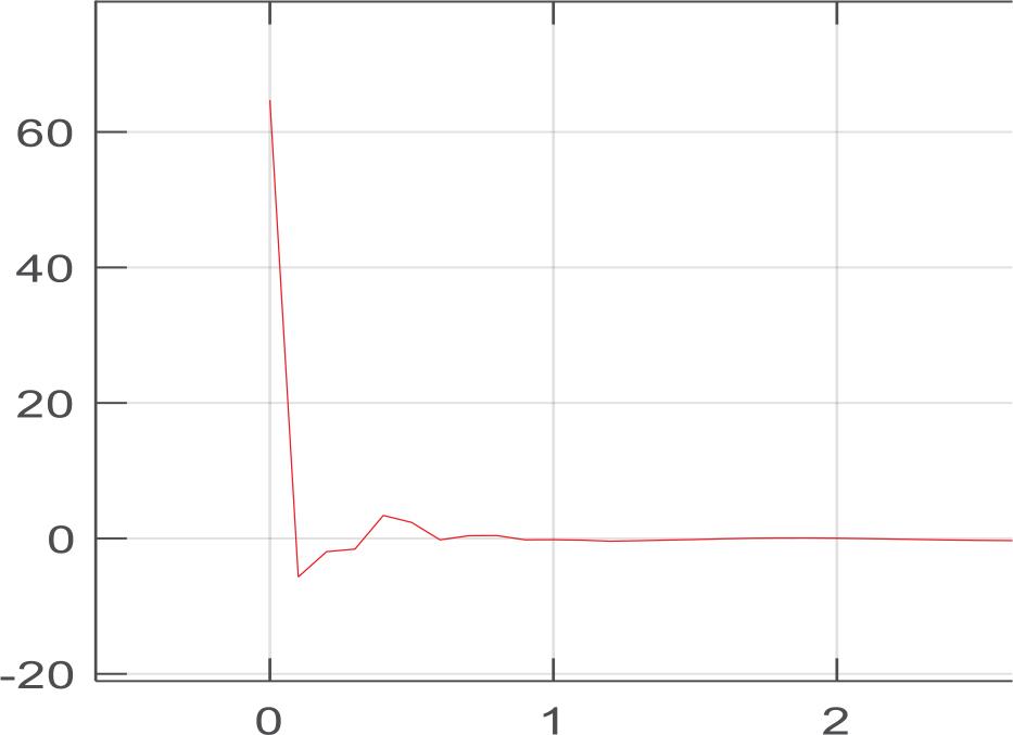
Figures 3 and 5 show an enlarged view of the first 5 seconds from the control signals.
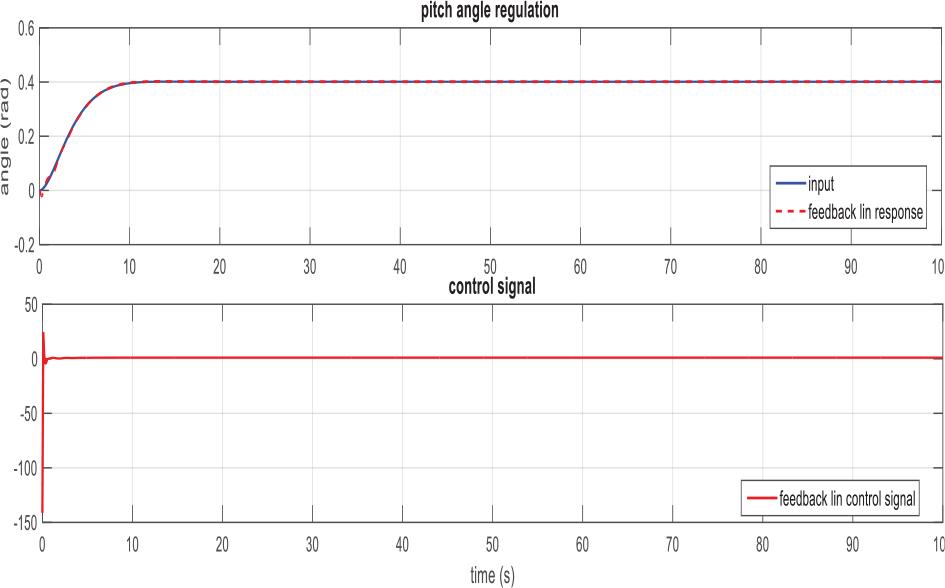
Pitch angle control by linearizing control in simulation
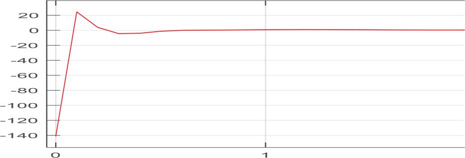
An enlarged view of the first 5 seconds of Figure 2
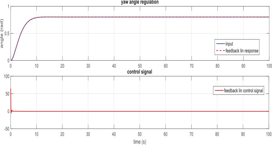
Yaw angle control by linearizing control in simulation
An enlarged view of the first 5 seconds of Figure 4
In the first mode of regulation (Figures 3 and 4), we note that the transient state is excellent without overshoot, and has a mean square error of order 10-4. The control signal was also excellent; note that there are peaks in the first fractions of a second in Figures 3 and 5, which is a typical phenomenon of control by feedback linearization. in practice, the actuator does not even notice because the problem is quickly corrected by the corrector, and we then notice a signal free of peaks and not noisy, visible from both angles.
- -
Trajectory tracking
In the second simulation, the model is excited by a sinusoidal input. The obtained results are presented in Figures 6 and 7.
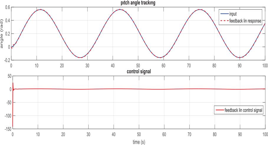
Trajectory tracking for the pitch angle controlled by the linearizing control in simulation
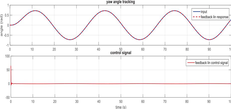
Trajectory tracking for yaw angle controlled by linearizing control in simulation
Regulation error values
| Feedback-lin | ||
|---|---|---|
| M-A of error | Pitch | MAE = 0.0100 |
| Yaw | MAE = 0.0060 | |
| M-S of error | Pitch | MSE = 6.6811e−04 |
| Yaw | MSE = 4.4122e−04 | |
Tracking error values
| Feedback-lin | ||
|---|---|---|
| MA of error | Pitch | MAE = 0.0066 |
| Yaw | MAE = 0.0023 | |
| MS of error | Pitch | MSE = 5.7529−05 |
| Yaw | MSE = 7.0992e−06 | |
This is to test its performance in trajectory tracking. This sinusoidal signal is characterized by:
- -
For the pitch: amplitude: 0.4, frequency: 0.2, centered at 0.2
- -
For yaw: amplitude: 0.8, frequency: 0.2, centered at 0.
For the second mode in Figures 6 and 7 – trajectory tracking – we noticed a tracking error trending towards zero. Given that the setpoint curve is exactly the same as the response curve, we can hardly differentiate them; with an optimal control signal and without noise, it is suitable for the actuators while respecting the specifications mentioned above.
Below are two tables containing the quadratic error and the absolute error between the setpoint and the response for the two modes.
In the simulation, we see that this controller has proven its effectiveness on this system, although it is complex and difficult to implement compared to the linear methods. In feedback linearization control, difficulties arise from the cascade of two laws of control: the inner control, which linearizes the system and depends on the physical state of the of the system, and the outer or auxiliary control, which stabilizes and provides performance in the closed loop. This control depends on the mathematical (linearized) state; if the inner control fails, the outer control can’t stabilize and give satisfactory performance in the closed loop.
The limitations of this scheme are:
- -
Non-robustness, because of the naivety of this command which is entirely based on the mathematical model of the system.
- -
Instability of the dynamics of zeros.
- -
Inapplicability to the non-linearizable class of non-linear systems.
By applying this method, we not only obtained the stability of the system, but also the performances, which were very excellent in accordance with the specifications.
In this subsection, we will implement the control laws directly in the real system to verify their robustness and efficiency in a real application.
Note at the beginning that the application of this nonlinear control on the TRMS allowed us to run the experiments from any initial set of conditions as long as they belonged to the basin of attraction of the system; the stability of the system was preserved, and the performances were similar.
We note from the results obtained in Figures 8 and 9 that we could not obtain satisfactory results in the pursuit, and we were therefore satisfied with the regulation. The same input used in the simulation has been inserted into the system. We applied a step disturbance on each angle to check its performance as well as its robustness in disturbance rejection. This disturbance was applied at the 50th second.
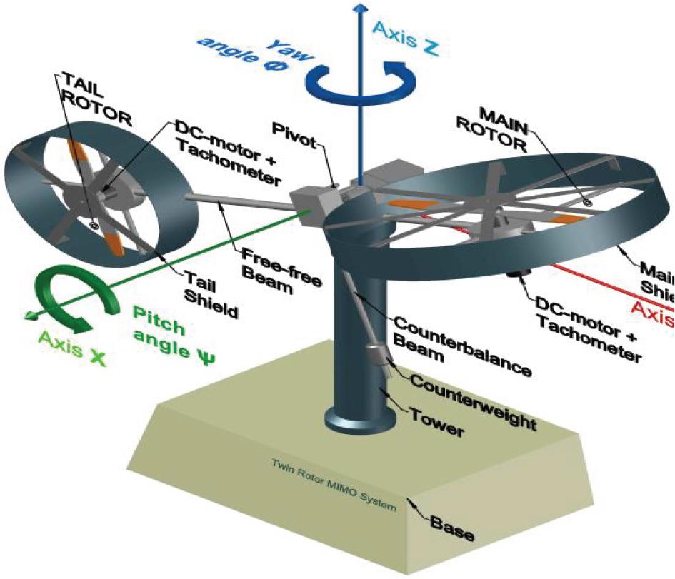
Diagram of the TRMS
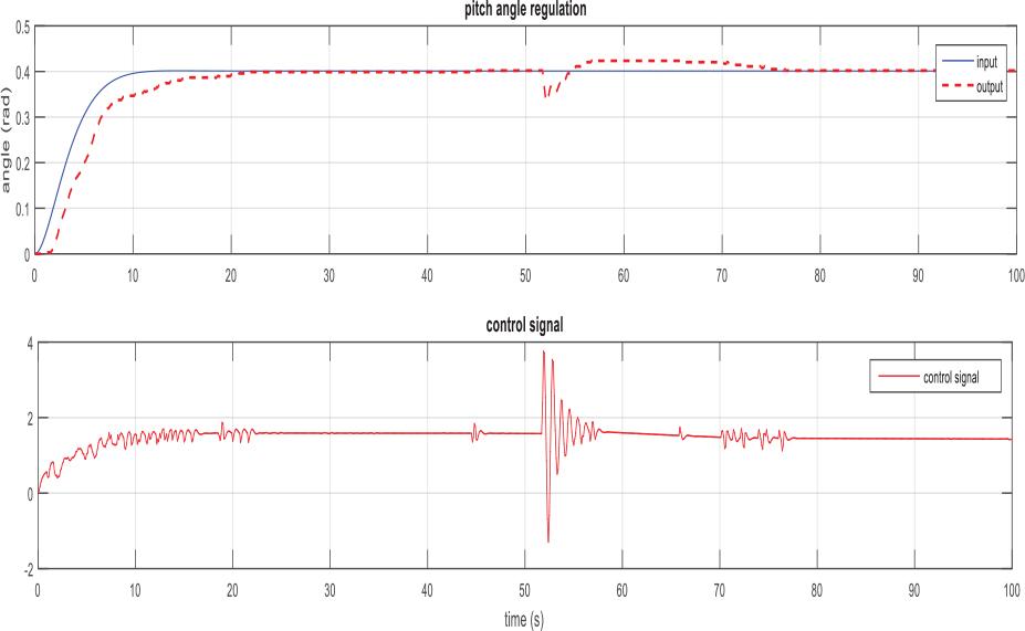
Pitch control by linearizing control in experiment
We note in Figures 9 and 10 presented above the results for the regulation are quite satisfactory, proving the stability of the system.
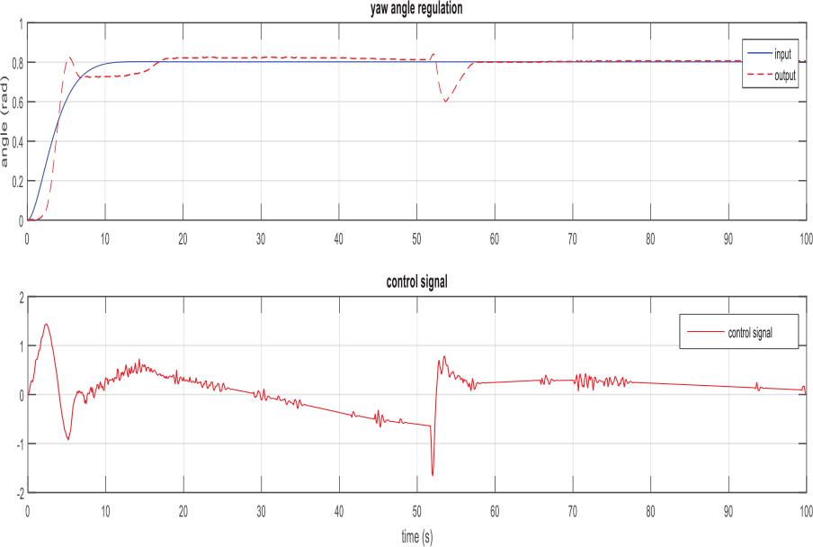
Experimental yaw control using the feedback linearizing control
The auxiliary controller also did its job by achieving the performance required in the specifications. For example, we mention that the response time is less than 4 seconds for the yaw angle, with an overshoot of less than 10%, and for the pitch angle, the response time is 3 seconds with an overshoot of 0%.
We also note the robustness of the control scheme in terms of rejection of disturbances and, in particular, performance. In terms of speed of rejection, it is approximately 3 seconds, with a small overshoot for the two angles and a clear performance for the yaw angle. Elsewhere, the steady state error is almost zero, thus improving accuracy.
In this paper, a nonlinear control based on global linearization and stabilization of the closed-loop system was developed and applied to TRMS. This strategy requires accessibility to all states of the system, which is not possible in the case of TRMS because this platform has only two sensors that measure pitch and yaw angles. This means an observer is required in order to implement this control. We have chosen a nonlinear observer the Thau observer, for its simplicity and efficiency. This has been proven by the satisfactory results obtained in regulation. A linear-state feedback system was used as an auxiliary control in order to stabilize the system and obtain the required performance.
It is concluded that this control yielded excellent results for the two objectives: regulation and enslavement. These results were quite satisfactory in real time for stability and regulation. For tracking, however it needs to be robust to reinforce stability, improve performance in regulation, and succeed in pursuit. This will be the main motivation for the next work. In nonlinear control, to implement an efficient tracking scheme, the control should be robust because the exact parameters used in the mathematical model of the system are not known. The main motivation for future work is to develop robust feedback linearization.