

Figure 1.
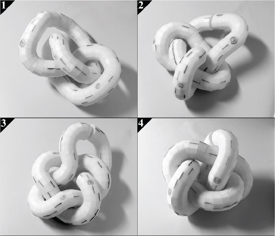
Figure 2.
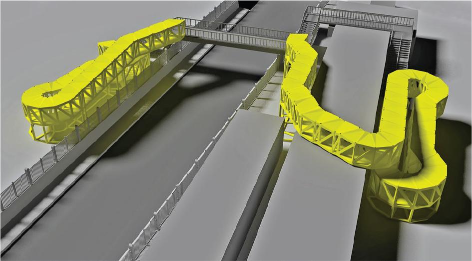
Figure 3.
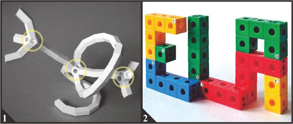
Figure 4.
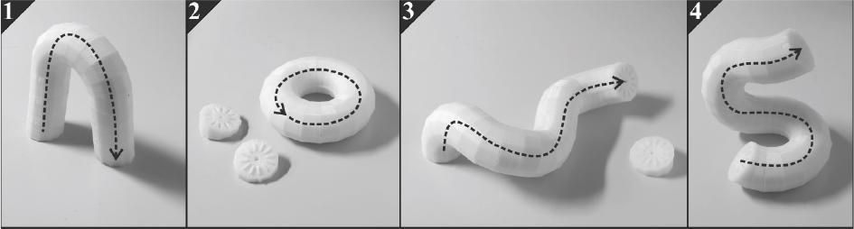
Figure 5.
Figure 6.
Figure 7.
Figure 8.
Figure 9.
Figure 10.
Figure 11.
Figure 12.
Figure 13.
Steps for creating an Extremely Modular System or its transformation
| Start | Transformation | Operator |
|---|---|---|
| General structure | ↴ | aS [Gi, (ii, BFi, ui)] |
| Add twigs | aT[Gi, ((p1, BF1, u1),(p2, BF2, u2),…,(pk, BFk, Uk))] | |
| Remove branches | rB [Gi, ((p1, BF1), (p2, BF2), …,(pi, BFk))] | |
| Substructure @ buds | ↲ | |
| ↴ | ||
| ↓ | Displace branches | dB[Gi, (((pi, BFi),(pj, BFj)),…)] |
| Units @ branches | ↲ | |
| ↴ | ||
| ↓ | Add units @ branches | aU[Gi,((p1,BF1,(v11,l11),…,(vk1,lk1)),…,(pj,BFj,(v1j,l1j),…,(vkj,lkj)))] |
| Remove units @ branches | rU[Gi,((p1,BF1,(l11,…,lk1),…,(pJ,BFJ,(l1j,…,lkJ)))] | |
| Invert units @ branches | iU[Gi ((p1,BF1,(l11,…,lk1),…,(pj,BFj,(l1j,…,lkj)))] | |
| End | ↲ |