
Construction automation deals with applying the principles of industrial automation to the construction sector or in the prefabrication of construction components.
Extremely Modular System (EMS for short) is a relatively new concept introduced a few years ago in [1]. It represents a new approach to the design of engineering structures and architectural objects where the assembly of congruent units allows for the creation of free-form shapes.
The main difference from the traditional modular systems used in engineering and building construction is the emphasis on the minimal diversity of types of modules, ideally—just one. This is why these systems are extremely modular.
These are five basic advantages of EMSs:
- 1)
Economical – as they are suitable for mass fabrication, thus lowering the cost, so they can be broadly applied;
- 2)
Functional – as they allow for reconfiguration, expansion, reduction;
- 3)
Robust – since every module that fails can be easily replaced with an identical but functional one;
- 4)
Discrete – as they are suitable for intelligent mathematical modeling, and their configurations can be subjected to discrete (multi-objective) optimization using efficient search algorithms;
- 5)
Uniform – this feature is advantageous for rapid deployment and automated assembly.
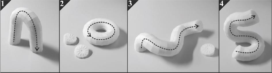
Pipe-Z (PZ) is a more fundamental system introduced in [2]. Its purpose was to form spatial mathematical knots by assembly of one type of unit (PZM), as shown in Fig. 1.
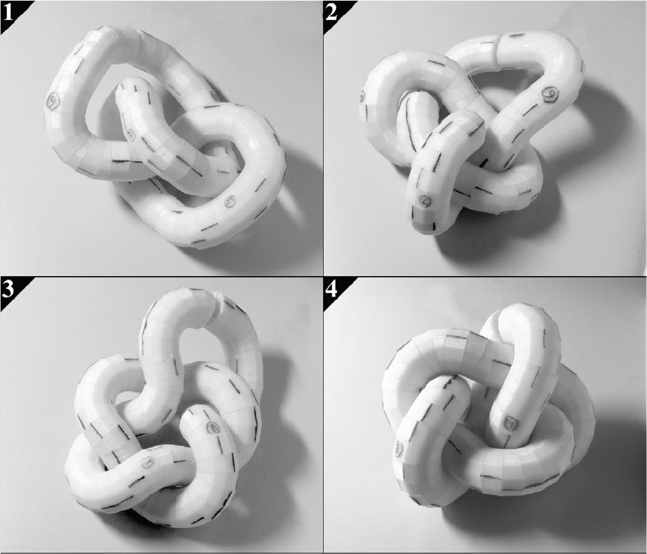
Physical models of mathematical prime knots constructed with extremely modular Pipe-Z: 1) Trefoil (31); 2) Figure-eight knot (41); 3) Cinquefoil (51); 4) 63 knot
The shape of PZ is controlled by the relative twists of congruent modules in a sequence.
Truss-Z (TZ) is a skeletal-frame hybrid construction system introduced in [3] for creating free-form pedestrian ramps and ramp networks connecting any number of terminals in space. TZ is composed of four variations of a single basic module subjected to affine transformations (mirror reflection, rotation, and combination of both). Figure 2 shows an example of TZ.
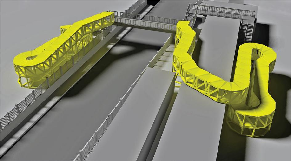
A computer rendering of an existing overpass retrofitted with two branches of Truss-Z, comprised of 47 modules on the left and 77 modules on the right
Although originally Pipe-Z allows for the creation of single-branched structures, by the introduction of an additional “branching buds,” it is also possible to construct multi-branched structures. Such a system is called EMS-2; an example based on PZ with an additional dodecahedron branching bud is shown in Figure 3.1.
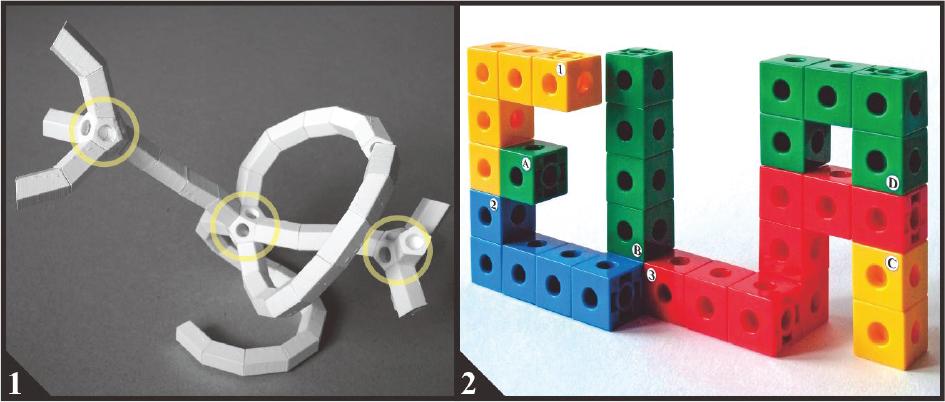
1) A physical model of the spatial multi-branch structure based on PZ. The bud is based on a truncated pentagonal prism. Three additional “branching buds” based on a dodecahedron (12-gon) are indicated by yellow circles. This system is called PZ12* and is considered EMS-2. 2) An example ofa spatial multi-branch quasi-EMS. This structure is built with “Space-Cube”—a system of toy blocks based on the simplest space-filling polyhedron—the cube. This system is called SC3 for short
The basic elements for both EMS and qEMS are the units. They are added sequentially along the direction of the construction, as illustrated with PZ in Figure 4.
Examples of 3D PZ structures. The units have been added sequentially at various twists along the dotted arrow. 1) An arch; 2) a torus; 3&4) free-form pipes
The core of the EMS concept is the shape of the unit, which allows the creation of various forms depending on its relative rotation. Its angular direction is relative to the directions of the branches, that is stems or twigs. For clarity all the following examples are reduced to 2D. Figure 5 shows examples of unit assembly for EMS and for the projection of SC3 to 2D, called SC2.
- 1)
TZ is a strict EMS. By rotation, the basic unit can be added in two ways, determining the shape of the structure. 1 and 0 turn right and left along the direction of the structure, respectively. 2) SC2 : the basic unit of this qEMS can be added in three ways: at the right, front, and left face, as indicated by numbers 1, 2, and 3, respectively.
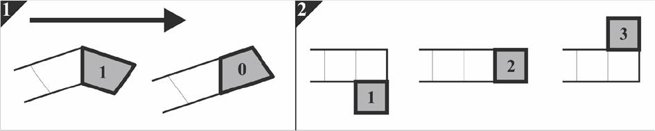
Planar projections of EMS (1) and qEMS (2)
In genetic algorithms, all candidate solutions have sets of properties encoded in so-called genotypes, usually as binary strings, arrays, trees, lists, or matrices, which can be mutated and/or altered [6].
A phenotype is an actual EMS with its (physical) form and structure encoded in a given genotype. Obviously, there is a bijection (one-to-one correspondence) between the set of genotypes and phenotypes.
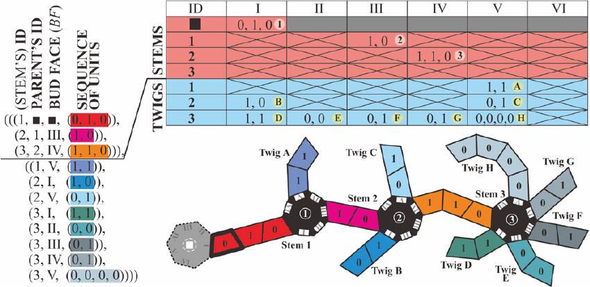
Figure 6 illustrates the nature-inspired naming for the components ofan EMS phenotype and parts of the corresponding genotype, which is a simple nested list.
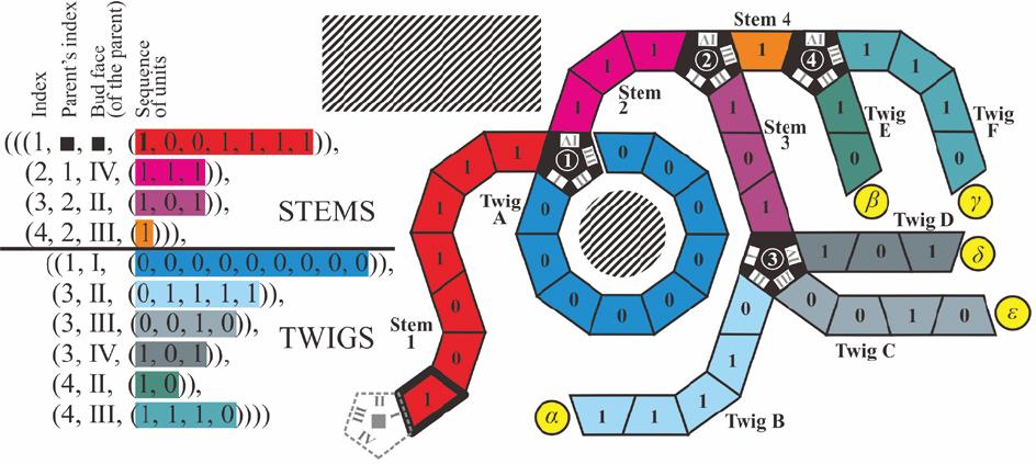
The nomenclature and encoding of EMS-2. On the left: the genotype (((1, ■, ■, (1, 0, 0, 1, 1, 1, 1)), (2, 1, IV, (1, 1, 1)), (3, 2, II, (1, 0, 1)), (4, 2, III, (1))), ((1, I, (0, 0,0,0,0,0,0,0,0)),(3,II,(0,1,1,1,1)),(3,III,(0,0,1, 0)), (3, IV, (1, 0, 1)), (4, II, (1, 0)), (4, III, (1, 1, 1, 0)))) tabulated for clarity. On the right: the corresponding phenotype. The obstacles are indicated by hatched areas. The terminals are indicated by Greek letters. In this case, the buds have a form of pentagons (indicated by black). Buds and bud faces are indexed with Arabic and Roman numerals, respectively. The corresponding elements are shown in the same colors. Stems and twigs are shown in “reddish” and “bluish” colors, respectively. The first unit is indicated by a thick black outline. It starts from the “virtual” unit shown by a gray dotted line
As illustrated in Figure 5, EMS-2 is comprised of
As mentioned in the Introduction, plesiohedra [4] are not considered as EMSs. The cube is the only regular solid that is also a plesiohedron [5]. Nevertheless, the multi-branched structures built with space-filling polyhedra can also be encoded in the same way. Figure 7 shows the genotype of the 2D projection (SC2) of the cube-based qEMS structure (SC3) shown in Figure 2.2.
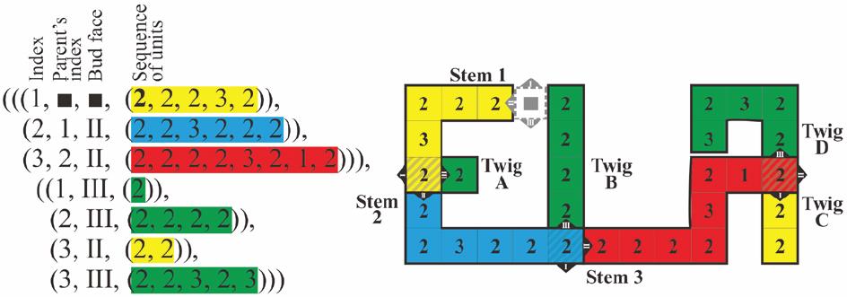
SC2: the 2D projection of SC3 structure shown in Figure 3.2. The genotype is shown on the left, and the corresponding phenotype is shown on the right. The respective corresponding elements are shown in the same colors. The last unit of each stem functions as a bud and is indicated by a diagonal hatch
As Figures 3 and 4 indicate, the hierarchical structures of EMS (and quasi-EMS) are defined as follows:
- i.
In general, the structure is constructed with branches.
- ii.
Branches are: stems and twigs.
- iii.
Stems end with buds. Twigs do not have buds
- iv.
Buds can have any number of faces (BFs)
- v.
A branch can be connected only to a bud.
- vi.
A stem has at least one unit. In the case of a one-unit long stem, it becomes a bud.
- vii.
Stems must not form closed loops.
- viii.
The first stem is connected to a “virtual” bud.
- ix.
The first stem is also rooted to the initial terminal. There are no more stems directly attached to a terminal.
- x.
A terminal can only be reached by a twig,% exclusive of the first stem and terminal.
Genotype of an ith Extremely Modular System Gi is encoded as a sequence of branches. The sequence of branches included two sub-sequence of stems and twigs:
Moreover, sj is a jth stem from the sequence of stems Si encoded in the following way:
fj is the index of the face of the parent’s bud (to which the jth stem is connected), and u is the sequence of units that constitute the jth stem
Units u depend on the type of EMS. E.g., for the systems shown in Figures 3.1 and 3.2: u ∈ (0, 1) and u ∈ (1, 2, 3), respectively. Buds also depend on the type of EMS. E.g., Truss-Z and SC3 do not have additional units for buds.
In Truss-Z, buds are constructed by reflecting the last unit in the stem sequence across the longer base of the trapezoidal unit.
In SC3, the last unit in a stem serves as a branching bud. On the other hand, the buds for EMS-2 systems can have any shape. In the examples shown in Figures: 3.1, 6 and 8 & 9 they are: dodecahedron, pentagon and heptagon, respectively.
From the left: the genotype; top right: the corresponding tabulated genotype; on the bottom right: the corresponding phenotype
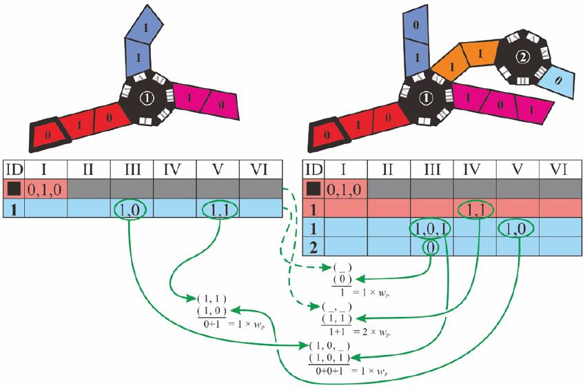
Calculation of the difference between two exemplary genotypes. The differences for all corresponding branches are summed up and multiplied by the penalty weight wP. Missing corresponding branches are indicated by dashed arrows. The difference between the two empty lists is 0
Since the first stem does not have a parent, p1, and f1 are dummies (blank).
The kth twig from the sequence Ti is defined in the following way:
fk, is the index of the face of the parent’s bud (to which the kth twig is connected), uk is the sequence of units that constitute the kth twig.
There is a full analogy between the list of twigs and stems.
There are seven operators collected in Table 1 that allow the construction of any EMS or the transformation of any EMSA to any other EMSB.
Steps for creating an Extremely Modular System or its transformation
| Start | Transformation | Operator |
|---|---|---|
| General structure | ↴ | aS [Gi, (ii, BFi, ui)] |
| Add twigs | aT[Gi, ((p1, BF1, u1),(p2, BF2, u2),…,(pk, BFk, Uk))] | |
| Remove branches | rB [Gi, ((p1, BF1), (p2, BF2), …,(pi, BFk))] | |
| Substructure @ buds | ↲ | |
| ↴ | ||
| ↓ | Displace branches | dB[Gi, (((pi, BFi),(pj, BFj)),…)] |
| Units @ branches | ↲ | |
| ↴ | ||
| ↓ | Add units @ branches | aU[Gi,((p1,BF1,(v11,l11),…,(vk1,lk1)),…,(pj,BFj,(v1j,l1j),…,(vkj,lkj)))] |
| Remove units @ branches | rU[Gi,((p1,BF1,(l11,…,lk1),…,(pJ,BFJ,(l1j,…,lkJ)))] | |
| Invert units @ branches | iU[Gi ((p1,BF1,(l11,…,lk1),…,(pj,BFj,(l1j,…,lkj)))] | |
| End | ↲ |
In addition, four operators for the population-based algorithm are defined and listed below.
Random genotype generator
Fix genotype
s is the desired number of stems,
t is the desired number of twigs,
l is the number of units generated randomly in additional branches, if applicable.
Tabulate genotype
This function transcribes genotype Gi into matrix T[Gi] with respect to the buds. See Figure 8 for an illustrative example.
Compare (tabulated) genotypes
Normalization here means that T[Gj] and T [Gk] have the same general structure. For example, if the dimensions of these genotypes differ, dummy elements are added. Moreover, C[Gj, Gk] ≥ 0.
Δ sums up the differences between the bit-strings of respective branches of the compared genotypes. Figure 9 illustrates the way how Δ is calculated.
Finally, four types of mutation and their combination have been defined as follows:
where is the gk is the kth genotype, mi is the normalized intensity of mutation, so that for 0 there is no displacement and for 1 all branches are displaced.
in this case, mi is normalized so that for 0, no units are added, and for 1, the number of units is doubled. Loci for the added units are distributed randomly among the branches. The values of the added units are random integers: 0 or 1.
Unlike stems, twigs can have zero length. Here, mi is normalized so that for 0, no unit is removed, and for 1, all units but one randomly selected unit per stem are removed. The loci for units to be removed are distributed randomly among the branches.
where mi is normalized, so that for 0 there is no change to any unit, and for 1 the values of all units are inverted. The loci for units to be inverted are distributed randomly among the branches.
where mi is the normalized intensity of mutation,
M randomly selects the mutation type according to parameters wdb, waU, wrU, and wiU, which are the normalized weights (from 0 to 1) for corresponding mutations: MdB, MaU, MrU, and MiU.
Evolution Strategy is a classic nature-inspired heuristic method introduced in [7].
Unlike other evolutionary algorithms, it does not employ recombination but only intensive mutation. For a review of the literature on this method, see [8].
This experiment is a two-objective
- 1)
Create a layout of a multi-branch Truss-Z (MTZ).
- 2)
There are six terminals at given locations: the initial terminal (Ts), and five aligned terminals T1…T5, as shown in Figure 15.
- 3)
The (initial) direction of the first unit is given at Ts.
- 4)
The number of units is to be
minimal . - 5)
The reaching error (rE) is to be
minimal (explained below).
Reaching error (rE) is the sum of distances between each terminal and respective twig tips, as illustrated in Figure 10.
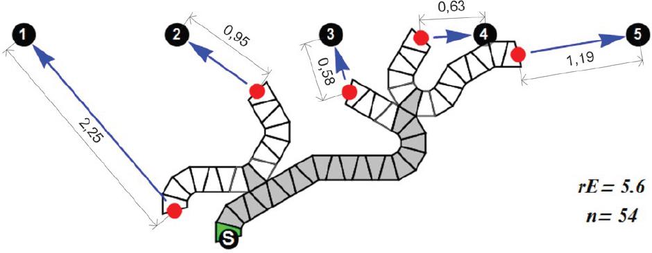
In this case, reaching error rE = 2.25 + 0.95 + 0.58 + 0.63 + 1.19 = 5.6. The number of units n = 54. Stems with branching units are indicated in gray. Twigs are white
The cost function CF for a given ith multi-branch Truss-Z (MTZi) with m number of destination terminals is calculated as follows:
The initial population is generated randomly using rG operator described above. However, it is rational to start from the most reasonable initial population by using certain observations. E.g., the number of twigs must be exactly 5. This is because only twigs can reach the terminals, and there are five of them. However, with the number of stems it is not so obvious. Figure 11 shows four different allowable MTZ configurations connecting five terminals with the initial terminal TS.
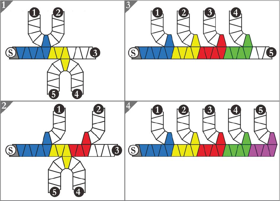
Sub-figures 1, 2, 3, and 4 show allowable MTZs connecting five terminals with: 2, 3, 4, and 5 stems, respectively
Therefore, the number of stems in every candidate solution must be within the range [2,5]. The initial population of 200 MTZs has been generated with the following parameters:
the number of twigs: tmin = tmax = 5;
the number of units in each branch: umin = 5, umax = 15.
Several trials at various combinations of parameters have been performed. Each experiment has been terminated after 100 iterations. Figure 12 shows the best phenotypes in the final trial.
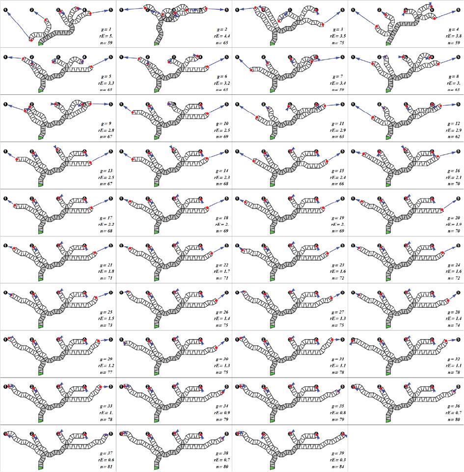
The final trial of the Evolution Strategy-based experiment. For each phenotype, the generation number (g), the reaching error (rE), and the number of units (n) are shown in the bottom right corner. There has been no further improvement after 39 generations. Stems with branching units are indicated in gray. Twigs are white
As Figure 12 indicates, in the beginning, several individuals were infeasible due to self-intersection. Nevertheless, relatively soon, this problem disappeared, as gradually the feasible offspring were produced by infeasible parents. Figure 13 shows the final solution and its three-dimensional interpretation.
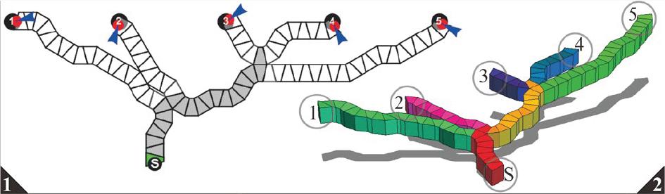
1) The best MTZ layout produced by Evolution Strategy. 2) The three-dimensional MTZ based on this layout
The concept of hierarchical structures has been outlined in the context of Extremely Modular Systems. The biology-inspired nomenclature, genetic encoding, and operations for this class of structures have been explained and illustrated.
Although the evolution strategy-based algorithm presented here has not been optimized for efficiency, it shows relatively good convergence. For more information on this approach, see [9].