
Table 1
Overview of the ten hybrid GSHP studies reviewed.
| REFERENCE | LOCATION | CLIMATE | BUILDING | SYSTEM |
|---|---|---|---|---|
| Pardo et al. (2010) | Valencia (ES) | Mediterranean | Office building | GSHP+ASHP+storage |
| X. Wang et al. (2010) | Harbin (CN) | Severe cold | Detached house | Solar+GSHP seasonal |
| You et al. (2014) | 3 cities (CN) | Cold | Hotel | GSHP+AHCa |
| You et al. (2015) | Harbin (CN) | Severe cold | Hotel | GSHP+AHCa |
| Emmi et al. (2017) | Vicenza (IT) | Temperate | Detached house | PVT+GSHP+ASHP |
| Grossi et al. (2018) | Bologna (IT) | Temperate | Detached house | DSHPb dual-source |
| Zheng et al. (2022) | Changsha (CN) | Hot summer | Dormitory | PV+GSHP+ASHP |
| Li et al. (2024) | Handan (CN) | Cold | Residential complex | PVT+GSHP+ASHP |
| F. Wang et al. (2024) | Harbin (CN) | Severe cold | Office building | BIPV/Tc+energy piles |
| Yue et al. (2025) | Qingdao (CN) | Cold | Gymnasium | PVT+GSHP+ASHP+battery |
[i] aAHC: aerothermal heat compensator. bDSHP: dual-source heat pump. cBIPV/T: building-integrated PV/thermal.
Table 2
Performance results and ground temperature drift reported across the ten studies. “ΔT soil” refers to the inter-annual ground temperature change (negative = cooling); values after a slash indicate the stabilised value with the hybrid system active. LCC: life-cycle cost; ALCC: annualised life-cycle cost.
| REFERENCE | COP syst. | ΔT soil | ECON. METRIC | KEY FINDING |
|---|---|---|---|---|
| Pardo et al. (2010) | 3.8 | N/A | Best payback | Elec. –60% vs ASHP |
| X. Wang et al. (2010) | 6.55 | +2 K | – | Solar = 50% of heat |
| You et al. (2014) | 2.9–4.7 | –12.7 K/stable | Sav. 5–6% | COP 4.1→2.0 w/o AHC |
| You et al. (2015) | 4.5–15 | –11.2 K/stable | Sav. 23.9% | Fails yr 7 w/o AHC |
| Emmi et al. (2017) | 3.55–3.94 | –2.5 K (stable) | N/A | PVT+air compet. w/o ground |
| Grossi et al. (2018) | 3.1–3.5 | –4.5 K/stable | BHE –30–50% | APF opt. depends on BHE |
| Zheng et al. (2022) | 4.69 | –6.3 K/stable | ALCC –8% | COP 3.2→2.9 |
| Li et al. (2024) | 3.8–6.0 | –1.4 K | ASHP cheaper | Medium-deep 1,500 m |
| F. Wang et al. (2024) | 2.96–3.02 | +0.7 K (stable) | LCC –57–62% | Conv. stops yr 11 |
| Yue et al. (2025) | 6.3 | –2.9 K/+0.1 K | LCC –55% | Elec. –71% |
Table 3
Economic parameters for LCOE computation.
| PARAMETER | VALUE | UNIT |
|---|---|---|
| Drilling cost (equipped borehole) | 120 | EUR/m |
| GSHP cost | 600 | EUR/kW |
| ASHP cost | 600 | EUR/kW |
| Electricity price | 230 | EUR/MWh |
| Weighted average cost of capital (WACC) | 4 | % |
| Analysis horizon | 10 | years |
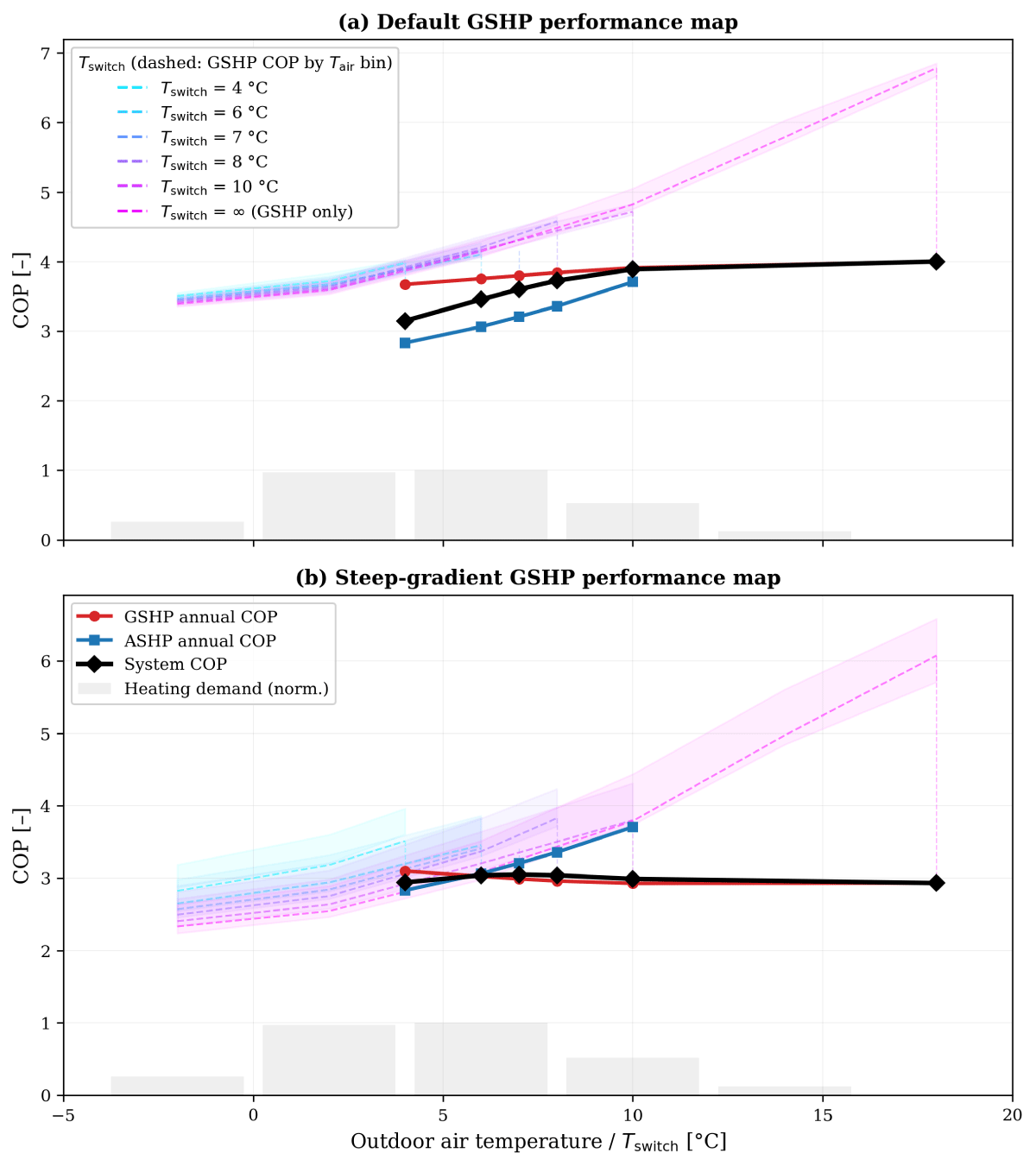
Figure 1
System, GSHP and ASHP annual COP as a function of the switching temperature. Dashed curves show the GSHP COP per outdoor air temperature bin (one curve per Tswitch); shaded bands indicate the interquartile range. Grey bars represent the normalised heating demand distribution by temperature bin. Top (a): default GSHP performance map. Bottom (b): steep-gradient GSHP performance map.
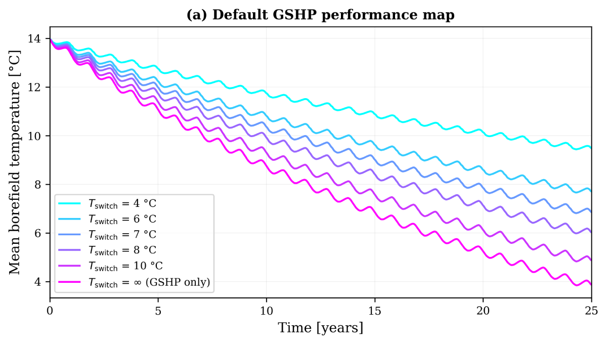
Figure 2
Monthly-averaged borefield temperature over 25 years for each switching temperature (Langres, 1,000 kW, default performance map). Lower Tswitch values preserve the ground temperature by limiting geothermal extraction.
Table 4
Optimal hybrid configurations—Montpellier. For each building (rows) and available surface ratio (column groups), the retained configuration minimises LCOE while satisfying Tfluid ∈ [–3°C, 40°C].
| CONFIG. | SURFACE 100% | SURFACE 70% | SURFACE 50% | ||||||||||||
|---|---|---|---|---|---|---|---|---|---|---|---|---|---|---|---|
| d | TSW | COP | LCOE | d | TSW | COP | LCOE | d | TSW | COP | LCOE | ||||
| % | m | °C | %ref | % | m | °C | %ref | % | m | °C | %ref | ||||
| 500 kW, 0% HL | 70 | 12.2 | 8 | 3.80 | 92.3 | 70 | 10.2 | 8 | 3.79 | 92.3 | 80 | 8.0 | 8 | 3.80 | 99.9 |
| 500 kW, 20% HL | 80 | 11.2 | 11 | 4.74 | 93.5 | 80 | 9.3 | 10 | 4.58 | 95.6 | 90 | 7.4 | 11 | 4.77 | 99.9 |
| 1000 kW, 0% HL | 80 | 11.2 | 11 | 4.47 | 90.8 | 70 | 10.0 | 8 | 3.81 | 90.8 | 80 | 7.9 | 8 | 3.81 | 97.8 |
| 1000 kW, 20% HL | 80 | 11.2 | 11 | 4.76 | 93.0 | 80 | 9.3 | 10 | 4.59 | 95.1 | 80 | 7.9 | 8 | 4.13 | 100.8 |
| 2000 kW, 0% HL | 70 | 12.0 | 8 | 3.82 | 91.1 | 70 | 10.0 | 8 | 3.82 | 91.1 | 80 | 7.9 | 8 | 3.82 | 98.3 |
| 2000 kW, 20% HL | 80 | 11.2 | 10 | 4.60 | 95.4 | 80 | 9.4 | 8 | 4.14 | 101.1 | 80 | 7.9 | 8 | 4.15 | 101.1 |
[i] n/nref: borehole count vs. reference; d: borehole spacing; Tsw: switching temperature; COP: global system COP (heating + cooling); LCOE: relative to reference geothermal installation (100% = same cost). HL: cooling-to-heating load ratio.
Table 5
Optimal hybrid configurations—Langres. Same conventions as Table 4.
| CONFIG. | SURFACE 100% | SURFACE 70% | SURFACE 50% | ||||||||||||
|---|---|---|---|---|---|---|---|---|---|---|---|---|---|---|---|
| d | TSW | COP | LCOE | d | TSW | COP | LCOE | d | TSW | COP | LCOE | ||||
| % | m | °C | %ref | % | m | °C | %ref | % | m | °C | %ref | ||||
| 500 kW, 0% HL | 70 | 11.9 | 6 | 3.46 | 85.2 | 70 | 10.0 | 4 | 3.13 | 89.2 | 80 | 7.9 | 4 | 3.13 | 96.3 |
| 500 kW, 20% HL | 70 | 11.9 | 6 | 3.85 | 88.2 | 70 | 10.0 | 4 | 3.51 | 92.8 | 80 | 7.9 | 6 | 3.87 | 94.3 |
| 1000 kW, 0% HL | 70 | 12.0 | 6 | 3.46 | 85.7 | 70 | 10.0 | 4 | 3.14 | 89.5 | 80 | 7.9 | 4 | 3.14 | 96.8 |
| 1000 kW, 20% HL | 70 | 12.0 | 6 | 3.86 | 88.8 | 70 | 10.0 | 4 | 3.54 | 93.2 | 80 | 7.9 | 4 | 3.55 | 100.1 |
| 2000 kW, 0% HL | 70 | 12.0 | 7 | 3.64 | 83.5 | 70 | 10.0 | 4 | 3.17 | 88.6 | 80 | 7.9 | 4 | 3.17 | 96.4 |
| 2000 kW, 20% HL | 70 | 12.0 | 7 | 3.92 | 85.0 | 70 | 10.0 | 6 | 3.77 | 86.6 | 80 | 7.9 | 6 | 3.77 | 94.1 |
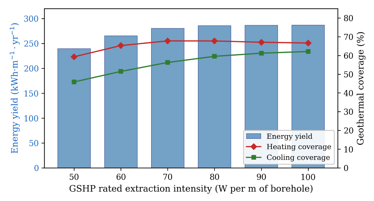
Figure 3
Effect of GSHP rated extraction intensity on 10-year average energy yield and geothermal coverage (Montpellier, 1,000 kW, 60% cooling ratio, 20 boreholes at 200 m).
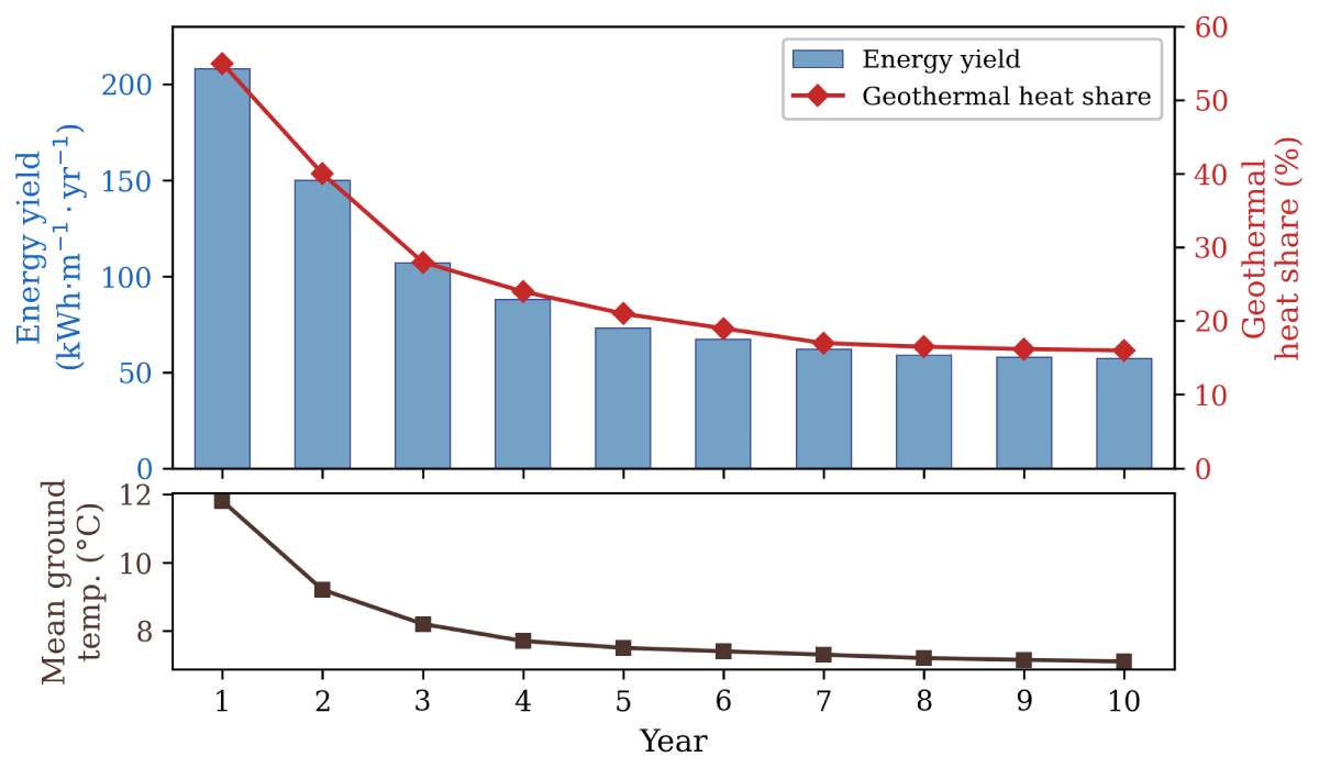
Figure 4
Annual performance degradation of the base-load hybrid system (Langres, 1,000 kW, heating only, 20 boreholes at 200 m). Top: energy yield (bars) and geothermal heat share (line). Bottom: mean borefield temperature.
Table 6
Base-load hybrid system performance (10-year average, 1,000 kW, 20 boreholes at 200 m). The ref row gives the GSHP-only reference for direct comparison. HL: cooling-to-heating load ratio; d: borehole spacing; yield: energy delivered per metre of borehole per year; fh, fc: geothermal heating and cooling coverage.
| CONFIGURATION | d(m) | YIELD kWh/m/yr | COP syst. | fh(%) | fc (%) | LCOE EUR/MWh |
|---|---|---|---|---|---|---|
| Montpellier (GSHP 80 W/m = 320 kW) | ||||||
| 0% HL, ref | 10 | 42 | 4.84 | 100 | – | 352 |
| 0% HL, hybrid | 12 | 149 | 3.65 | 54 | – | 208 |
| 0% HL, hybrid | 8 | 120 | 3.51 | 44 | – | 210 |
| 20% HL, ref | 10 | 61 | 4.93 | 100 | 100 | 281 |
| 20% HL, hybrid | 12 | 207 | 3.94 | 61 | 71 | 180 |
| 20% HL, hybrid | 8 | 188 | 3.86 | 54 | 71 | 181 |
| 60% HL, ref | 10 | 92 | 5.02 | 100 | 100 | 233 |
| 60% hybrid | 12 | 289 | 4.20 | 70 | 58 | 147 |
| 60% HL, hybrid | 8 | 286 | 4.19 | 68 | 60 | 147 |
| Langres (GSHP 200 kW) | ||||||
| 0% HL, ref | 10 | 37 | 4.11 | 100 | – | 364 |
| 0% HL, hybrid | 12 | 128 | 2.81 | 32 | – | 176 |
| 0% HL, hybrid | 8 | 93 | 2.72 | 23 | – | 178 |
| 20% HL, ref | 10 | 58 | 4.32 | 100 | 100 | 279 |
| 20% HL, hybrid | 12 | 219 | 3.21 | 42 | 61 | 151 |
| 20% HL, hybrid | 8 | 195 | 3.15 | 36 | 61 | 152 |