
1 Introduction
Ground Source Heat Pumps (GSHPs) exploit the thermal stability of the shallow subsurface to deliver annual coefficients of performance (COPs) of 3.5–5.0, well above those of Air Source Heat Pumps (ASHPs) in most European climates (ADEME, 2023; Staffell et al., 2012). In France, field measurements report average GSHP COPs of 4.3 versus 2.9 for ASHPs (ADEME, 2023). Despite this advantage, the French market remains heavily skewed toward air source: about one million ASHP units are sold annually versus fewer than 5,000 GSHPs (AFPG, 2024). The primary barrier is economic: vertical borehole heat exchangers (BHEs) represent 40–60% of total GSHP capital expenditure (Grossi et al., 2018; International Energy Agency, 2022), with equipped borehole costs in France of EUR 80/m to EUR 120/m (ADEME & BRGM, 2021). The International Energy Agency (2022) also estimates learning rates of 18% for ASHP versus only 3.3% for GSHP, implying that the cost gap is likely to widen over time.
Beyond initial cost, the long-term viability of GSHP systems depends on the thermal balance of the borefield. In heating-dominated climates, annual heat extraction exceeds injection, causing a progressive decline in ground temperature. You et al. (2014) reported a 12.7 K drop over 10 years at Harbin (China), leading to a 52% COP reduction; You et al. (2015) observed system failure after 7 years without correction; and F. Wang et al. (2024) showed that a conventional energy-pile system ceases operation after 11 years. The typical impact is about 3% COP loss per kelvin of ground cooling. To sustain long-term extraction, boreholes must be oversized or spaced further apart, creating a diminishing-returns dynamic.
Hybrid Ground Source Heat Pump (HGSHP) systems address these limitations by coupling the GSHP with one or more auxiliary sources, most commonly an ASHP, to reduce geothermal extraction and relax borefield sizing constraints. Several architectures have been investigated, including hybrid GSHP–ASHP systems with alternating monovalent operation (Grossi et al., 2018; Pardo et al., 2010), solar-assisted configurations (Emmi et al., 2017; F. Wang et al., 2024; X. Wang et al., 2010), and multi-source systems with photovoltaic-thermal (PVT) collectors, storage, and batteries (Yue et al., 2025; Zheng et al., 2022). The GSHP–ASHP and GSHP–PVT options are the most studied; among them, GSHP–ASHP is particularly attractive for dense tertiary contexts, requiring little additional footprint and offering a markedly lower cost per kW than solutions involving additional drilling.
Grossi et al. (2018) demonstrated a key counter-intuitive result: the annual performance factor (APF) of a dual-source heat pump (DSHP) is not maximised by exclusive ground-source operation, but rather exhibits an optimum at a specific air-ground switching temperature (Tswitch) that depends on borefield size. With undersized BHE fields (43–50% of reference), the DSHP achieves APF values 10–20% above a standalone ASHP while reducing borehole length by 30–50%.
Despite these promising results, significant gaps remain in the literature. First, the body of HGSHP research is dominated by Chinese studies with drilling costs (EUR 10/m to EUR 32/m) that are not representative of the European context (EUR 80/m to EUR 120/m). Second, the three European studies analysed (Emmi et al., 2017; Grossi et al., 2018; Pardo et al., 2010) report only isolated economic indicators and never address borefield size reduction within a systematic methodological framework. Third, and perhaps most notably, none of the ten studies reviewed formulates the borefield optimisation problem in terms of the fluid temperature operating limits (–3°C to 40°C), which constitute the binding technical and regulatory constraint for real installations. Finally, no existing study covers large-scale tertiary installations (500 kW to 2,000 kW) under French climatic conditions.
This paper addresses these gaps through three contributions:
An investigation of the COP optimisation potential of alternating monovalent GSHP–ASHP operation, extending the Grossi et al. (2018) approach to large-scale installations and examining the sensitivity to heat pump performance data;
A parametric study of borefield size reduction under explicit fluid temperature constraints (–3°C to 40°C), quantifying LCOE improvements for 500 kW to 2,000 kW tertiary buildings in two French climates;
A base-load hybrid model where the GSHP operates continuously and the ASHP provides backup, removing the constraint that the GSHP must cover peak load alone, and introducing the energy yield per metre of borehole as the key economic metric.
2 Literature review
A systematic search on ScienceDirect, targeting experimental and simulated hybrid geothermal installations with aerothermal coupling, yielded ten relevant studies spanning 2010–2025 (Table 1).
Table 1
Overview of the ten hybrid GSHP studies reviewed.
| REFERENCE | LOCATION | CLIMATE | BUILDING | SYSTEM |
|---|---|---|---|---|
| Pardo et al. (2010) | Valencia (ES) | Mediterranean | Office building | GSHP+ASHP+storage |
| X. Wang et al. (2010) | Harbin (CN) | Severe cold | Detached house | Solar+GSHP seasonal |
| You et al. (2014) | 3 cities (CN) | Cold | Hotel | GSHP+AHCa |
| You et al. (2015) | Harbin (CN) | Severe cold | Hotel | GSHP+AHCa |
| Emmi et al. (2017) | Vicenza (IT) | Temperate | Detached house | PVT+GSHP+ASHP |
| Grossi et al. (2018) | Bologna (IT) | Temperate | Detached house | DSHPb dual-source |
| Zheng et al. (2022) | Changsha (CN) | Hot summer | Dormitory | PV+GSHP+ASHP |
| Li et al. (2024) | Handan (CN) | Cold | Residential complex | PVT+GSHP+ASHP |
| F. Wang et al. (2024) | Harbin (CN) | Severe cold | Office building | BIPV/Tc+energy piles |
| Yue et al. (2025) | Qingdao (CN) | Cold | Gymnasium | PVT+GSHP+ASHP+battery |
[i] aAHC: aerothermal heat compensator. bDSHP: dual-source heat pump. cBIPV/T: building-integrated PV/thermal.
2.1 Hybrid architectures and performance
The dominant hybridisation scheme couples a GSHP with an ASHP as auxiliary heat source. The switching logic between sources varies:
Temperature-based switching: Grossi et al. (2018) introduced a fixed outdoor air switching temperature Tswitch: when the outdoor air temperature is below Tswitch, the DSHP operates in ground-source mode; above it, in air-source mode. This monovalent alternating strategy is the simplest to implement and constitutes the baseline for the present study. Pardo et al. (2010) used a similar priority-based approach with GSHP as primary source (COP 4.5 vs 2.5 for ASHP).
Seasonal or calendar-based switching: Li et al. (2024) used ASHP alone in early/late season, GSHP alone in mid-winter, and a 2/3–1/3 split in the coldest months. You et al. (2015) operated an aerothermal heat compensator (AHC) to transfer heat from air to ground during off-season.
COP-based real-time selection: Emmi et al. (2017) implemented a multi-source controller selecting at each timestep the source with the highest COP (air, ground, or PVT).
Differential signal: Zheng et al. (2022) used a ΔTsoil–air > 1 K criterion to switch between GSHP and ASHP.
Several studies integrate photovoltaic-thermal (PVT) collectors to provide a triple benefit: electricity generation, thermal recharge of the ground, and PV cell cooling (Emmi et al., 2017; F. Wang et al., 2024; Yue et al., 2025). X. Wang et al. (2010) demonstrated seasonal thermal storage using solar collectors injecting heat into the ground from spring to autumn.
Table 2 summarises the main performance indicators. System COPs span a wide range, driven by climate, building type, and system complexity. The high values reported in solar-assisted or PV-coupled studies only count grid-supplied electricity in the denominator and are not directly comparable to a thermodynamic COP. The results provide a useful comparative basis but are difficult to synthesise given the diversity of metrics and cost assumptions: drilling costs range from EUR 10/m to EUR 32/m in Chinese studies to EUR 50/m in Grossi et al. (2018) (Italy) and EUR 80/m to EUR 120/m in France.
Table 2
Performance results and ground temperature drift reported across the ten studies. “ΔT soil” refers to the inter-annual ground temperature change (negative = cooling); values after a slash indicate the stabilised value with the hybrid system active. LCC: life-cycle cost; ALCC: annualised life-cycle cost.
| REFERENCE | COP syst. | ΔT soil | ECON. METRIC | KEY FINDING |
|---|---|---|---|---|
| Pardo et al. (2010) | 3.8 | N/A | Best payback | Elec. –60% vs ASHP |
| X. Wang et al. (2010) | 6.55 | +2 K | – | Solar = 50% of heat |
| You et al. (2014) | 2.9–4.7 | –12.7 K/stable | Sav. 5–6% | COP 4.1→2.0 w/o AHC |
| You et al. (2015) | 4.5–15 | –11.2 K/stable | Sav. 23.9% | Fails yr 7 w/o AHC |
| Emmi et al. (2017) | 3.55–3.94 | –2.5 K (stable) | N/A | PVT+air compet. w/o ground |
| Grossi et al. (2018) | 3.1–3.5 | –4.5 K/stable | BHE –30–50% | APF opt. depends on BHE |
| Zheng et al. (2022) | 4.69 | –6.3 K/stable | ALCC –8% | COP 3.2→2.9 |
| Li et al. (2024) | 3.8–6.0 | –1.4 K | ASHP cheaper | Medium-deep 1,500 m |
| F. Wang et al. (2024) | 2.96–3.02 | +0.7 K (stable) | LCC –57–62% | Conv. stops yr 11 |
| Yue et al. (2025) | 6.3 | –2.9 K/+0.1 K | LCC –55% | Elec. –71% |
Ground temperature drift ranges from mild (about –4.5 K in 15 years at Bologna and stabilising thereafter (Grossi et al., 2018)) to catastrophic (–12.7 K in 10 years at Harbin (You et al., 2014)), with system shutdown reported by both You et al. (2015) (after 7 years) and F. Wang et al. (2024) (after 11 years) in the absence of mitigation. Most articles analyse the ground temperature decline, but the economic necessity of controlling it is rarely studied directly, except in extreme cold climates.
2.2 Identified gaps
Three gaps emerge from this review.
First, none of the ten studies formulates the borefield optimisation problem in terms of fluid temperature operating limits (–3°C to 40°C in France). In practice, this constraint is the binding criterion for borefield sizing: it determines the minimum number and spacing of boreholes required for a given extraction profile.
Second, the three European studies (Emmi et al., 2017; Grossi et al., 2018; Pardo et al., 2010) emphasise COP over costs. They report isolated economic indicators (a payback time in Pardo et al. (2010), a normalised borehole reduction in Grossi et al. (2018)), but none performs a detailed economic optimisation, and none treats borefield size reduction within a systematic framework. Paradoxically, it is in Europe—where drilling costs are highest—that this perspective is most critical. The Chinese studies (F. Wang et al., 2024; Yue et al., 2025; Zheng et al., 2022) do present formalised economic optimisations, but with cost assumptions that are not transferable to Europe.
Third, no existing study covers large-scale tertiary installations (500 kW to 2,000 kW) under French climatic conditions.
This study addresses these three gaps through a parametric LCOE analysis with French cost assumptions, explicit fluid temperature constraints, and building capacities of 500 kW to 2,000 kW.
3 Methodology
3.1 Building models and climatic data
The case studies are well-insulated office buildings (new construction, envelope U-value 0.7 W/(m² · K)) modelled with the TRNSYS Type 56 multizone component. Three design heating capacities are considered: 500 kW, 1,000 kW, and 2,000 kW—the latter corresponding to the French regulatory threshold for géothermie de minime importance. Two representative French climates are selected via Typical Meteorological Year (TMY) data: Montpellier (Mediterranean, mild winters) and Langres (semi-continental, harsh winters). For each climate and building size, three cooling-to-heating demand ratios are simulated: 0%, 20%, and 60% (the latter excluded for Langres). The heating setpoint is 19°C; the cooling setpoint is adjusted to achieve the target ratio. The envelope assumes 50% glazing, 2 vol/h air renewal during occupancy, and standard internal gains.
3.2 TRNSYS simulation model
The system is implemented in TRNSYS 17 (Klein et al., 2010). The building uses Type 56 (multizone) with thermal demand computed from setpoint temperatures and weather data.
Ground heat exchanger Vertical BHEs are modelled with Type 557b (duct ground heat storage) (Hellström, 1991). Parameters include borehole depth (200 m reference), diameter, grout conductivity, U-tube geometry, soil thermal conductivity (2 W/(m · K)), volumetric heat capacity (2.16 MJ/(m3 · K)), and undisturbed ground temperature (mean annual air temperature from TMY). These soil thermal properties are reasonably homogeneous across metropolitan France, so no sensitivity analysis was performed on them. The hexagonal borehole layout has been verified against analytical g-functions from open-source Python library pygfunction (Cimmino, 2018), agreeing within 0.5 K on brine outlet temperature over 25 years.
Heat pumps The GSHP and ASHP are modelled with TRNSYS Type 927 and Type 941, normalised performance maps. The nominal heating COP is 5 at 10°C/35°C for the GSHP, and 4 at 7°C/35°C for the ASHP. Each unit operates on/off; capacity modulation is achieved by varying the number of units active at each timestep.
3.3 Hybridisation models
Two hybridisation control mechanisms are used in this work, both aimed at containing the brine temperature swing but acting on different timescales.
Alternating monovalent (T-switch), used in Sections 4 and 5. Inspired by Grossi et al. (2018): only one heat source is active at a time. The GSHP runs alone below Tswitch, the ASHP runs alone above, and the GSHP also handles all cooling (dedicated cooling emitters are assumed installed). The GSHP is sized for the full peak heating load. This caps the annual ground extraction implicitly, which is well suited to conventionally sized or moderately reduced borefields, but ties borehole count to peak power rather than to annual energy.
Brine-temperature hysteresis controller (base-load), used in Section 6. Both heat pumps can operate, with the GSHP in base load and the ASHP in backup. The GSHP shuts off when the brine reaches the regulatory limits (–3/+40°C) and restarts after a hysteresis recovery. This controller acts only when the brine temperature actually leaves the allowed range, so it does not preventively limit the long-term ground temperature drift; it does, however, allow the GSHP to be sized well below peak load and the borefield to be deliberately undersized, in order to maximise the annual energy yield per metre of borehole and therefore the economic amortisation of the drilling investment.
3.4 Reference borefield sizing
The reference borefield for each building configuration is sized as follows:
Borehole depth: 200 m;
Borehole spacing: 10 m (5% of depth);
Number of boreholes: minimum number ensuring that the brine temperature remains within –3°C to 40°C over a 25-year simulation;
Hexagonal layout, confirmed by comparison with pygfunction as described above.
This reference case represents a conventionally sized geothermal installation: it is the minimum borefield that satisfies the regulatory fluid temperature limits over the 25-year horizon at a standard 10 m spacing, and it is the benchmark against which the hybrid configurations are compared.
3.5 Optimisation problem formulation
The fluid temperature constraint Tfluid ∈ [–3°C, 40°C] is the central feasibility condition. The brine temperature is governed by two interacting factors:
Short-term variation (dominant): swings of 10 K or more over a few hours, combining the temperature drop at the borehole wall under recent extraction intensity (strongest under sustained high-power extraction) with the instantaneous brine–wall ΔT required to drive the heat exchange;
Inter-annual ground temperature drift: a slow drift of the mean borefield temperature driven by the cumulative heating/cooling imbalance and borefield geometry.
Even without inter-annual drift, short-term variation alone imposes a minimum total borehole length; additional boreholes provide margin against the drift, spread over enough area to limit thermal interference.
Minimising the LCOE under the fluid-temperature constraint implicitly maximises the energy extracted per metre of borehole, since the drilling cost is amortised over the GSHP-delivered energy. This metric—the borehole energy yield—is used as an explicit indicator in Section 6 to show how the base-load model raises it well above conventional geothermal sizing. Two horizons are used: simulations run over 25 years (the French Fonds Chaleur (ADEME) eligibility horizon, on which fluid-temperature feasibility is verified), while the LCOE horizon is 10 years (typical investment-decision timeframe for tertiary owners). Each subsequent result indicates which horizon applies.
3.6 Parametric study design
For each building configuration and surface availability ratio (50%, 70%, 100% of the reference borefield surface), the sensitivity analysis explores two degrees of freedom:
Borehole count ratio: 70%, 80%, 90%, or 100% of the reference number of boreholes;
Switching temperature Tswitch: six values from a climate-specific list (lower values for Langres than Montpellier).
The borehole spacing is derived from the number of boreholes and the available surface area, with a minimum spacing of 7.5 m. For each combination, a 25-year hourly TRNSYS simulation is run. The retained hybrid configuration for each (building, surface ratio) pair is the one achieving the lowest LCOE while satisfying the fluid temperature constraint. Approximately 1,000 simulations were executed in total.
3.7 Economic assumptions
The economic parameters are summarised in Table 3. The drilling cost of EUR 120/m is the fully equipped borehole cost (drilling, high-density polyethylene (HDPE) double-U probe, bentonite-cement grouting, head connection), consistent with French market data for deep boreholes (ADEME & BRGM, 2021). Heat-pump costs reflect large-scale tertiary installations and may be conservative for MW-scale systems. The electricity tariff includes taxes and network charges for tertiary consumers.
Table 3
Economic parameters for LCOE computation.
| PARAMETER | VALUE | UNIT |
|---|---|---|
| Drilling cost (equipped borehole) | 120 | EUR/m |
| GSHP cost | 600 | EUR/kW |
| ASHP cost | 600 | EUR/kW |
| Electricity price | 230 | EUR/MWh |
| Weighted average cost of capital (WACC) | 4 | % |
| Analysis horizon | 10 | years |
The LCOE combines capital expenditure (CAPEX) and operating expenditure (OPEX):
where H = 10 years is the LCOE horizon, r = 4 % is the WACC, Qt is the annual thermal energy delivered, and OPEXt includes electricity consumption and maintenance.
3.8 Simulation framework
A custom Python framework manages the study: TRNSYS deck generation, parallel execution (~5 min per 25-year simulation), and KPI extraction (COP, geothermal coverage, LCOE, fluid temperature extremes). Approximately 1,000 simulations were executed in total.
4 COP optimisation through hybridisation
Even when the borefield is sized to cover the full load on its own, alternating monovalent hybridisation may still improve the system COP by limiting ground temperature depletion: switching part of the heating load to the ASHP preserves a higher GSHP COP during operation and may raise the overall system performance. Grossi et al. (2018) report an optimum Tswitch where this trade-off is balanced. We test the same mechanism here, with the GSHP performance map as the key sensitivity parameter. The borefield is sized at the minimum number of boreholes satisfying the –3°C brine constraint under pure-geothermal operation (Section 3.4); the case study is Langres, 1,000 kW peak heating, no cooling.
4.1 Simulation setup
Six values of the switching temperature are tested: Tswitch ∈ {4,6,7,8,10} °C plus the pure-geothermal reference (Tswitch = ∞); each is run as a 25-year hourly simulation. Two GSHP performance maps bracket the role of evaporator sensitivity:
Default map: the standard TRNSYS map (rated COP = 5 at 10°C/35°C), which yields COP = 3.0 at the 0°C/50°C regime—a typical value for a brine/water heat pump and our realistic reference scenario;
Steep-gradient map: same rated COP, but with a Carnot efficiency that drops more rapidly with the source/load spread, reaching COP = 1.7 at the 0°C/50°C regime. This map is not representative of any commercial heat pump; it serves as a sensitivity test for how steep the gradient would need to be for ground cooling to materially penalise GSHP operation.
4.2 Effect of switching temperature on system COP
Figure 1 shows, for each performance map, the annual GSHP COP, ASHP COP, and overall system COP as a function of the switching temperature. The dashed curves provide additional detail by plotting the GSHP COP per outdoor air temperature bin for each Tswitch, illustrating how ground cooling affects performance at each temperature level.
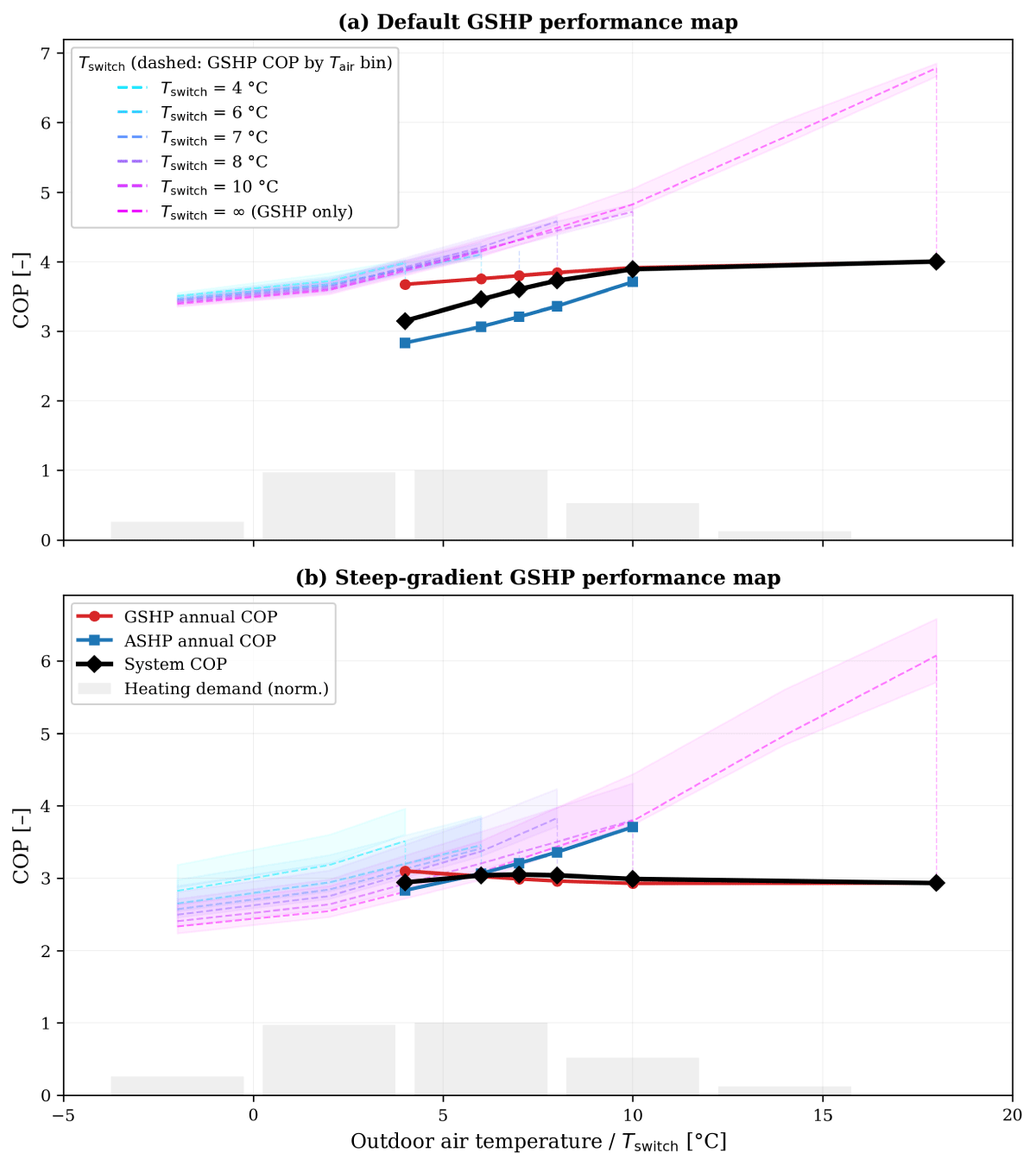
Figure 1
System, GSHP and ASHP annual COP as a function of the switching temperature. Dashed curves show the GSHP COP per outdoor air temperature bin (one curve per Tswitch); shaded bands indicate the interquartile range. Grey bars represent the normalised heating demand distribution by temperature bin. Top (a): default GSHP performance map. Bottom (b): steep-gradient GSHP performance map.
With the default map (Figure 1a), the system COP increases monotonically with Tswitch, from 3.15 at Tswitch = 4°C (44% geothermal coverage) to 4.00 for pure geothermal. No optimum is observed: peak performance is reached without any hybridisation. The GSHP annual COP stays in 3.67–4.00, while the ASHP annual COP rises from 2.83 (Tswitch = 4°C) to 3.71 (Tswitch = 10°C). With a realistic GSHP map, ground cooling does not erode the GSHP COP enough to offset the GSHP’s inherent advantage over the ASHP.
With the steep-gradient map (Figure 1b), the GSHP annual COP now decreases with Tswitch (3.10 at 4°C to 2.93 for pure geothermal), as ground cooling becomes much more penalising. A mild optimum appears around Tswitch = 6–7°C (COP ≈ 3.05), a +4% gain over pure geothermal—the mechanism reported by Grossi et al. (2018).
Recovering such an optimum thus requires a steeper COP–evaporator gradient than commercial brine/water maps exhibit, and even then, the gain is marginal. Under realistic performance assumptions, alternating monovalent hybridisation does not optimise the system COP: the case for hybridisation must therefore be made on the other levers explored in the remainder of the paper, namely the reduction of the borefield surface area (Section 5) and the base-load hybrid operating model (Section 6).
4.3 Ground temperature evolution
Figure 2 shows the monthly-averaged borefield temperature over 25 years for each Tswitch (default map). Pure-geothermal operation drifts by about 10 K (14 to 4°C), against 6 K at Tswitch = 4°C. Despite this large difference, the impact on the system COP is modest: the brine inlet temperature during extraction is dominated by the instantaneous extraction rate rather than the average ground temperature, and the peak-extraction GSHP COP penalty is similar across switching temperatures.
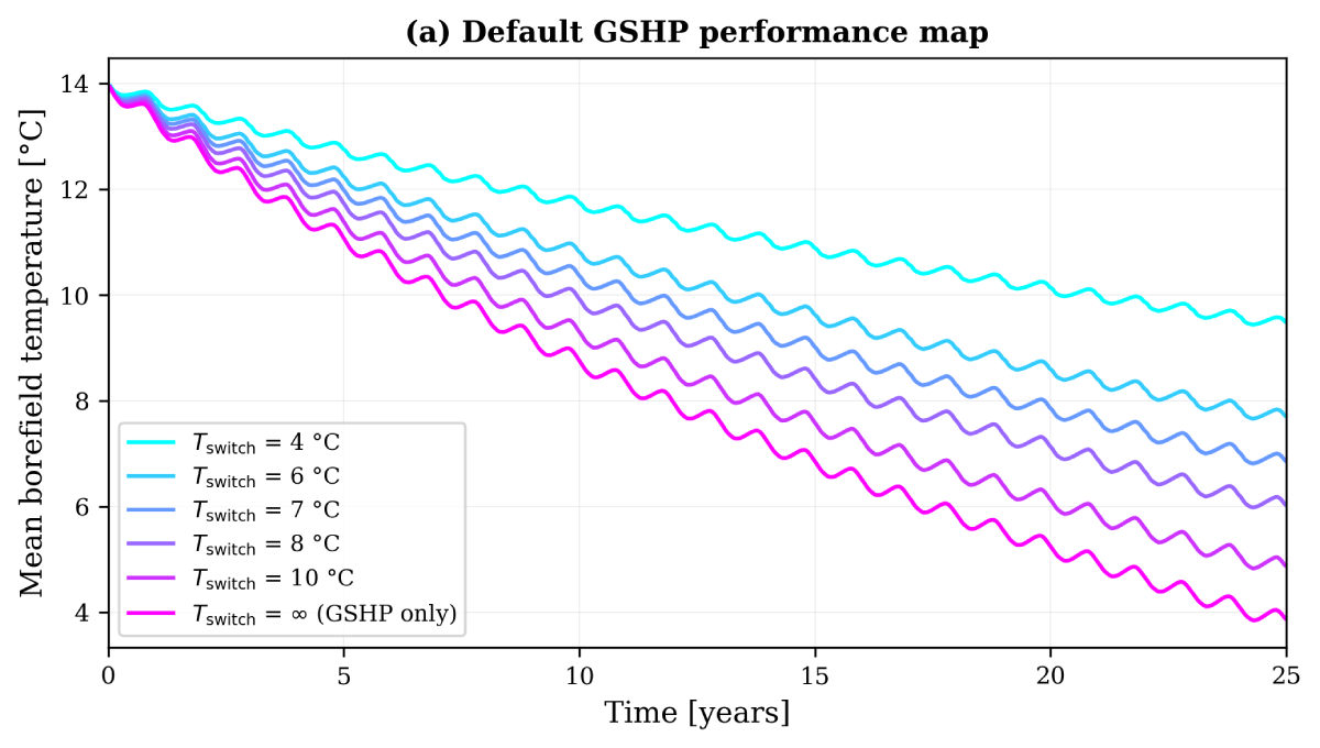
Figure 2
Monthly-averaged borefield temperature over 25 years for each switching temperature (Langres, 1,000 kW, default performance map). Lower Tswitch values preserve the ground temperature by limiting geothermal extraction.
The default TRNSYS normalised performance maps are retained for all subsequent analyses. The remaining sections explore the two other levers offered by hybridisation: the reduction of the borefield surface area (Section 5) and the base-load operating model (Section 6).
5 Borefield size reduction under fluid temperature constraints
Since COP optimisation through hybridisation is modest with standard performance maps, we now ask whether alternating monovalent hybridisation can enable a significant reduction in borefield surface area while maintaining acceptable system performance—a question directly relevant to urban and peri-urban sites where land availability is the primary barrier to geothermal deployment.
5.1 Methodology
For each building, the reference geothermal installation (Section 3.4) is deformed by reducing the available land area to 70% or 50%. Within each surface constraint, we sweep the borehole count ratio (70–100% of reference) and Tswitch, retaining the lowest-LCOE configuration that satisfies Tfluid ∈ [–3°C, 40°C].
For Montpellier with 60% cooling, the binding constraint is the maximum fluid temperature, not the minimum. Since alternating monovalent hybridisation does not reduce cooling-season injection, those cases are excluded below (surface reduction remains feasible if the borehole count is preserved). In this model the GSHP covers the full peak heating load alone, which limits the borefield load factor; Section 6 explores an alternative logic operating the GSHP as the base-load source.
5.2 Results
Tables 4 and 5 consolidate the optimal hybrid configurations for each building and surface ratio. For each case, the table reports the borehole count ratio (n/nref), borehole spacing, switching temperature, system COP, and LCOE relative to the reference geothermal installation.
Table 4
Optimal hybrid configurations—Montpellier. For each building (rows) and available surface ratio (column groups), the retained configuration minimises LCOE while satisfying Tfluid ∈ [–3°C, 40°C].
| CONFIG. | SURFACE 100% | SURFACE 70% | SURFACE 50% | ||||||||||||
|---|---|---|---|---|---|---|---|---|---|---|---|---|---|---|---|
| d | TSW | COP | LCOE | d | TSW | COP | LCOE | d | TSW | COP | LCOE | ||||
| % | m | °C | %ref | % | m | °C | %ref | % | m | °C | %ref | ||||
| 500 kW, 0% HL | 70 | 12.2 | 8 | 3.80 | 92.3 | 70 | 10.2 | 8 | 3.79 | 92.3 | 80 | 8.0 | 8 | 3.80 | 99.9 |
| 500 kW, 20% HL | 80 | 11.2 | 11 | 4.74 | 93.5 | 80 | 9.3 | 10 | 4.58 | 95.6 | 90 | 7.4 | 11 | 4.77 | 99.9 |
| 1000 kW, 0% HL | 80 | 11.2 | 11 | 4.47 | 90.8 | 70 | 10.0 | 8 | 3.81 | 90.8 | 80 | 7.9 | 8 | 3.81 | 97.8 |
| 1000 kW, 20% HL | 80 | 11.2 | 11 | 4.76 | 93.0 | 80 | 9.3 | 10 | 4.59 | 95.1 | 80 | 7.9 | 8 | 4.13 | 100.8 |
| 2000 kW, 0% HL | 70 | 12.0 | 8 | 3.82 | 91.1 | 70 | 10.0 | 8 | 3.82 | 91.1 | 80 | 7.9 | 8 | 3.82 | 98.3 |
| 2000 kW, 20% HL | 80 | 11.2 | 10 | 4.60 | 95.4 | 80 | 9.4 | 8 | 4.14 | 101.1 | 80 | 7.9 | 8 | 4.15 | 101.1 |
[i] n/nref: borehole count vs. reference; d: borehole spacing; Tsw: switching temperature; COP: global system COP (heating + cooling); LCOE: relative to reference geothermal installation (100% = same cost). HL: cooling-to-heating load ratio.
Table 5
Optimal hybrid configurations—Langres. Same conventions as Table 4.
| CONFIG. | SURFACE 100% | SURFACE 70% | SURFACE 50% | ||||||||||||
|---|---|---|---|---|---|---|---|---|---|---|---|---|---|---|---|
| d | TSW | COP | LCOE | d | TSW | COP | LCOE | d | TSW | COP | LCOE | ||||
| % | m | °C | %ref | % | m | °C | %ref | % | m | °C | %ref | ||||
| 500 kW, 0% HL | 70 | 11.9 | 6 | 3.46 | 85.2 | 70 | 10.0 | 4 | 3.13 | 89.2 | 80 | 7.9 | 4 | 3.13 | 96.3 |
| 500 kW, 20% HL | 70 | 11.9 | 6 | 3.85 | 88.2 | 70 | 10.0 | 4 | 3.51 | 92.8 | 80 | 7.9 | 6 | 3.87 | 94.3 |
| 1000 kW, 0% HL | 70 | 12.0 | 6 | 3.46 | 85.7 | 70 | 10.0 | 4 | 3.14 | 89.5 | 80 | 7.9 | 4 | 3.14 | 96.8 |
| 1000 kW, 20% HL | 70 | 12.0 | 6 | 3.86 | 88.8 | 70 | 10.0 | 4 | 3.54 | 93.2 | 80 | 7.9 | 4 | 3.55 | 100.1 |
| 2000 kW, 0% HL | 70 | 12.0 | 7 | 3.64 | 83.5 | 70 | 10.0 | 4 | 3.17 | 88.6 | 80 | 7.9 | 4 | 3.17 | 96.4 |
| 2000 kW, 20% HL | 70 | 12.0 | 7 | 3.92 | 85.0 | 70 | 10.0 | 6 | 3.77 | 86.6 | 80 | 7.9 | 6 | 3.77 | 94.1 |
5.3 Analysis
Surface reduction with moderate COP trade-off. The central result is that the borefield surface can be reduced to 50% of the reference while maintaining a system COP above 3.1 in all cases. At 70% surface, the COP reduction is typically 0.1–0.7 units. A lower COP for a given building reflects a more hybridised configuration (lower Tswitch, higher ASHP share) that trades modest COP for reduced drilling investment.
Climate effect on switching temperature. The optimal Tswitch is systematically lower for Langres (4°C to 7°C) than for Montpellier (8°C to 11°C). This reflects the heating demand distribution by outdoor temperature: in Langres, a larger share of demand falls at very cold temperatures, so a low Tswitch already captures most of the heating load on the geothermal side; a higher value would extend GSHP operation into mild hours that contribute little to annual demand. At 50% surface, Tswitch converges to the lower end of each range to limit extraction intensity. Spacing drops to ~7.9 m at 50% surface, still above the practical minimum of 7.5 m.
LCOE. At full surface availability, hybrid configurations achieve LCOE reductions of 5–17% relative to the reference, with the best results at Langres (83.5% for 2,000 kW, 0% HL). At 50% surface, the LCOE is within 0–4% of the reference: hybridisation transforms an infeasible scenario into a viable one at comparable cost. LCOE gains are larger for Langres, where the greater heating demand amplifies the benefit of borehole count reduction.
6 Base-load hybrid operating model
The alternating monovalent model caps the energy extracted per metre of borehole at about 100 kWh/(m · yr), whereas roughly 250 kWh/(m · yr) would be required to break even over 15 years at EUR 120/m drilling cost. We therefore consider a base-load hybrid model: GSHP in base, ASHP in backup when the borefield can no longer sustain extraction (controller defined in Section 3.3). The borefield is undersized to 20% of peak capacity (20 boreholes at 200 m for a 1,000 kW building, following the 50 W/m rule of thumb). The key metric is the borehole energy yield: thermal energy (heating + cooling) delivered by the GSHP per metre per year. The analysis covers the five 1,000 kW configurations (Montpellier 0%, 20%, 60% cooling; Langres 0% and 20%).
6.1 Controller binding regimes
Whether the controller binds on the short-term or long-term timescale depends on the configuration. In mild climates with balanced loads the borefield recovers between peaks, so the binding constraint is the short-term brine temperature swing. In cold climates with heating-only loads, progressive cooling shifts more of the operation to the ASHP over the years, so the binding constraint becomes the inter-annual ground temperature drift.
6.2 Effect of GSHP extraction intensity
For the most favourable configuration (Montpellier, 1,000 kW, 60% cooling), Figure 3 shows the effect of the GSHP rated extraction intensity (50 W/m to 100 W/m) on the 10-year average yield and geothermal coverage, for a fixed borefield of 20 boreholes. Yield rises from 240 kWh/(m · yr) at 50 W/m to 286 kWh/(m · yr) at 80 W/m, where a clear plateau is reached. Beyond 80 W/m the controller increasingly cuts GSHP operation due to fluid-temperature violations. At the plateau, the geothermal system covers 68% of heating and 60% of cooling demand.
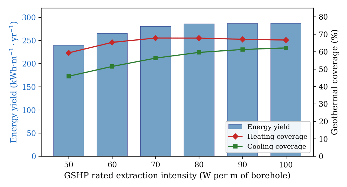
Figure 3
Effect of GSHP rated extraction intensity on 10-year average energy yield and geothermal coverage (Montpellier, 1,000 kW, 60% cooling ratio, 20 boreholes at 200 m).
6.3 Ground cooling as the limiting factor
In the most unfavourable configuration (Langres, 1,000 kW, heating only), inter-annual ground cooling constrains the intensive extraction strategy. Figure 4 shows the annual evolution over 10 years. Year-1 yield is 208 kWh/(m · yr) with 55% geothermal coverage; the mean ground temperature drops from 11.8°C to 7.1°C (ΔT = –4.7 K), and by year 10 yield falls to 57 kWh/(m · yr) (16% coverage). The controller is self-protecting: as the ground cools, the GSHP is cut off more often, converging to a regime where geothermal only contributes marginally. Combining the controller with a switching temperature (prioritising GSHP when air is cold) was tested but added only +3% system COP (2.67 to 2.75); this modest gain likely reflects the default TRNSYS ASHP map underestimating defrost losses at low air temperatures.
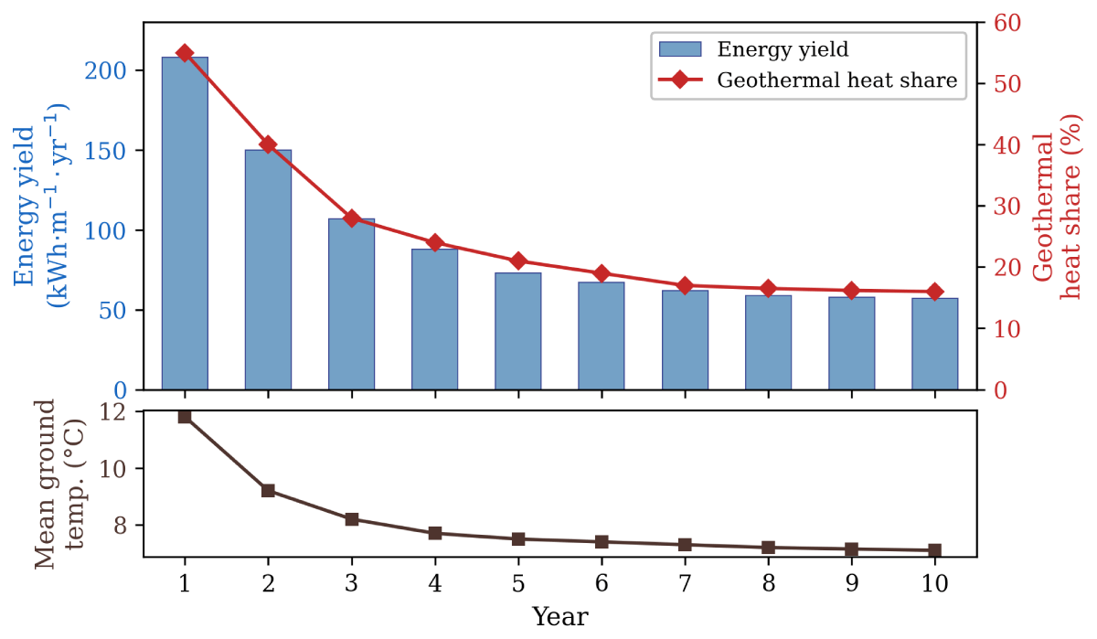
Figure 4
Annual performance degradation of the base-load hybrid system (Langres, 1,000 kW, heating only, 20 boreholes at 200 m). Top: energy yield (bars) and geothermal heat share (line). Bottom: mean borefield temperature.
6.4 Consolidated results across building configurations
Table 6 presents the 10-year averaged performance for all five building configurations; each tested with two borehole spacings (8 m and 12 m). All cases use 20 boreholes at 200 m. The GSHP is rated at 80 W/m (320 kW) for Montpellier (Section 6.2 plateau), and at 200 kW for Langres where ground cooling precludes higher intensities. Each configuration is compared against the GSHP-only reference of Section 5.
Table 6
Base-load hybrid system performance (10-year average, 1,000 kW, 20 boreholes at 200 m). The ref row gives the GSHP-only reference for direct comparison. HL: cooling-to-heating load ratio; d: borehole spacing; yield: energy delivered per metre of borehole per year; fh, fc: geothermal heating and cooling coverage.
| CONFIGURATION | d(m) | YIELD kWh/m/yr | COP syst. | fh(%) | fc (%) | LCOE EUR/MWh |
|---|---|---|---|---|---|---|
| Montpellier (GSHP 80 W/m = 320 kW) | ||||||
| 0% HL, ref | 10 | 42 | 4.84 | 100 | – | 352 |
| 0% HL, hybrid | 12 | 149 | 3.65 | 54 | – | 208 |
| 0% HL, hybrid | 8 | 120 | 3.51 | 44 | – | 210 |
| 20% HL, ref | 10 | 61 | 4.93 | 100 | 100 | 281 |
| 20% HL, hybrid | 12 | 207 | 3.94 | 61 | 71 | 180 |
| 20% HL, hybrid | 8 | 188 | 3.86 | 54 | 71 | 181 |
| 60% HL, ref | 10 | 92 | 5.02 | 100 | 100 | 233 |
| 60% hybrid | 12 | 289 | 4.20 | 70 | 58 | 147 |
| 60% HL, hybrid | 8 | 286 | 4.19 | 68 | 60 | 147 |
| Langres (GSHP 200 kW) | ||||||
| 0% HL, ref | 10 | 37 | 4.11 | 100 | – | 364 |
| 0% HL, hybrid | 12 | 128 | 2.81 | 32 | – | 176 |
| 0% HL, hybrid | 8 | 93 | 2.72 | 23 | – | 178 |
| 20% HL, ref | 10 | 58 | 4.32 | 100 | 100 | 279 |
| 20% HL, hybrid | 12 | 219 | 3.21 | 42 | 61 | 151 |
| 20% HL, hybrid | 8 | 195 | 3.15 | 36 | 61 | 152 |
Three findings emerge from these results.
Substantial LCOE reductions vs. the GSHP-only reference. The base-load model reduces the LCOE by 37–52% relative to the reference (e.g. 352 → EUR 208/MWh for Montpellier 0% HL, 364 → EUR 176/MWh for Langres 0% HL). Most of these savings come from the borefield being sized at 20% of the reference, with the bulk of the load served by the cheaper ASHP. Unlike a standalone ASHP, however, the hybrid keeps geothermal in the energy mix—with the associated non-economic benefits (load diversification, lower peak grid demand, building real-estate value).
Cooling loads unlock geothermal economic value. With at least 20% cooling demand, the yield reaches 188 kWh/(m · yr) to 219 kWh/(m · yr), and up to 289 kWh/(m · yr) at 60% cooling (Montpellier)—three to four times the GSHP-only reference yield (42 kWh/(m · yr) to 92 kWh/(m · yr)). The cooling season partially recharges the ground. Heating-only configurations achieve much lower yields (93 kWh/(m · yr) to 149 kWh/(m · yr)), confirming that thermal imbalance is the fundamental barrier in heating-dominated climates.
Borehole spacing matters under intensive extraction. 12 m spacing consistently raises the yield by 15–40% over 8 m, as intensive extraction amplifies thermal interference. Since the borefield is sized at only 20% of the reference, the absolute footprint remains compact even at 12 m spacing.
Where ground cooling limits the base-load approach, active recharge strategies (solar thermal or ASHP-driven summer recharge) could stabilise the borefield temperature and extend the applicability of the base-load model to heating-dominated climates—a direction discussed further in Section 7.3.
7 Discussion
7.1 Comparison with the literature
The borefield surface reductions of 30–50% achieved with the alternating monovalent model, with COP degradation limited to 0.1–0.7 units, are consistent with Grossi et al. (2018), who reported similar BHE length reductions for a residential DSHP in Bologna. The present study extends this finding to installations 50–200 × larger (500 kW to 2,000 kW vs. 8.6 kW), confirming the scalability of the hybrid approach. The LCOE improvements of 5–17% are comparable to the 8.1% ALCC reduction reported by Zheng et al. (2022), but achieved under European cost assumptions that are significantly less favourable to geothermal systems.
We do not, however, reproduce the hybridisation-driven gain on system performance reported by Grossi et al. (2018): under realistic performance assumptions the system COP is monotonic in Tswitch and maximised without hybridisation; a mild optimum only reappears with our steep-gradient sensitivity map.
The base-load model shifts the focus from borefield size to energy yield. The borehole yields of 188 kWh/(m · yr) to 289 kWh/(m · yr) obtained under balanced loads far exceed conventional geothermal sizing, confirming that the hybridisation logic itself—not just the borefield geometry—is a key economic lever. The rapid degradation in heating-only Langres (208 to 57 kWh/(m · yr) in 10 years) shows that ground cooling remains the fundamental limitation under imbalanced loads.
A distinctive feature of this study is the explicit treatment of the fluid temperature constraint as the binding feasibility condition: no prior study formulates borefield optimisation in these terms (Section 2.2), yet these limits drive both the reference sizing and the base-load controller thresholds.
7.2 Practical implications
For tertiary developers and operators, three takeaways emerge. Land-constrained sites: the alternating monovalent model enables geothermal deployment with 50% of the reference borefield surface, COP above 3.1 and LCOE within 0–4% of the unconstrained reference. Economic optimisation: the base-load model profitably uses geothermal as soon as cooling demand reaches 20%, and clearly benefits the borefield at 60% cooling, with 12 m spacing further improving extraction by 15–40%. Climate sensitivity: cold heating-only climates benefit most from surface reduction (up to –17% LCOE) but are least favourable for the base-load approach; balanced loads and mild climates offer the best conditions for both strategies.
7.3 Limitations and future work
The main limitations are: (i) heat-pump performance maps are default TRNSYS data, possibly under-representing COP degradation in the critical –3°C to 5°C evaporator range; (ii) the analysis is purely simulation-based, as in 8 of 10 studies reviewed; (iii) the 10-year LCOE horizon understates the value of the borefield as a >50-year asset; (iv) no sensitivity on cost parameters has been performed—the LCOE is dominated by CAPEX (79–87%), so drilling cost is the most influential parameter.
The main future-work direction is active ground recharge (solar thermal or ASHP-driven summer injection) to stabilise the borefield temperature in heating-dominated climates and establish the conditions under which hybrid systems consistently outperform standalone ASHP solutions.
8 Conclusion
This paper presents a parametric study of hybrid GSHP–ASHP systems for large-scale tertiary buildings (500 kW to 2,000 kW) in two French climates, using approximately 1,000 TRNSYS simulations over 25-year horizons with hourly resolution. The study addresses identified gaps in the literature: the absence of formalised economic analysis for European HGSHP systems, the lack of explicit fluid temperature constraints in borefield optimisation, and the absence of studies covering large-scale French installations.
The main conclusions are:
COP optimisation through alternating monovalent hybridisation is limited. With standard heat pump performance maps, the system COP varies by less than one unit across the range of switching temperatures tested. The result is sensitive to the COP gradient at low evaporator temperatures, which is poorly characterised in the open literature; under realistic assumptions we do not reproduce the hybridisation-driven optimum reported by Grossi et al. (2018).
Borefield surface can be halved while preserving cost and performance. Alternating monovalent hybridisation enables a 30–50% reduction in borefield surface area with system COP staying above 3.1 in all configurations tested (a trade-off of 0.1–0.7 COP units rather than a performance degradation), and even at 50% surface the LCOE remains within 0–4% of the unconstrained reference. This makes geothermal deployment feasible in land-constrained urban settings.
Alternating monovalent hybridisation reduces LCOE by 5–17% compared to a conventional geothermal installation at full surface availability, as the CAPEX reduction from fewer boreholes outweighs the increased ASHP electricity consumption. The gains are largest in cold climates (Langres: up to –17%).
Fluid temperature constraints are the binding design criterion. Formulating the borefield optimisation problem in terms of the regulatory fluid temperature limits (–3°C to 40°C) provides a physically meaningful and operationally relevant framework that is absent from the existing literature.
Base-load hybrid operation unlocks borefield profitability when cooling loads exist. With the GSHP in base load and the ASHP in backup, the energy yield per metre of borehole reaches 289 kWh/(m · yr) for 60% cooling demand, but remains limited by inter-annual ground cooling in heating-only cases. The corresponding LCOE reductions vs. the GSHP-only reference are substantial (40–50%), driven mainly by the undersized borefield and a larger ASHP share. The hybrid keeps geothermal in the mix (with its non-economic benefits), and active ground recharge could narrow the gap further.
Future work will focus on (i) active ground recharge strategies (solar thermal, ASHP-driven summer injection) to extend the base-load approach to heating-dominated climates, (ii) systematic multi-variable optimisation of borefield geometry and heat pump sizing, and (iii) improving the realism of heat pump performance data at low evaporator temperatures through manufacturer partnerships or experimental campaigns.
Additional File
The additional file for this article can be found as follows:
PowerPoint Slides
PowerPoint Slides relating to this article. DOI: https://doi.org/10.66506/essp.8-017-26.s1
Data Accessibility Statement
The TRNSYS deck templates and the Python orchestration framework are not publicly distributed, as their sharing is not permitted by the funders of the work. All technical and economic assumptions, building parameters, climate data and cost references are documented in Section 3 and in the bibliography, allowing the study to be reproduced with an independent TRNSYS implementation.
Author Contributions
The first author led the methodology, model implementation, results interpretation and manuscript drafting. The second author contributed geothermal expertise, supervised the project and verified the consistency and relevance of the results. Both authors approved the final version.
eceee paper ID
8-017-26