
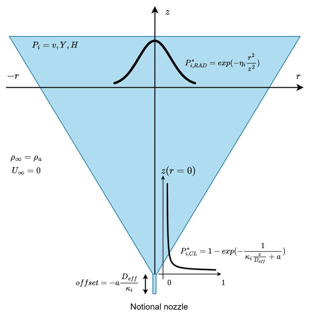
Figure 1
Schematic of scalar dissipation in an ideally expanded jet issued from a notional nozzle. Scalar decay can be described by a hyperbolic function along the axial direction and a Gaussian function along the radial direction (Kleinstein, 1964).
Table 1
Release conditions, measurement methods and centreline decay rates of past hydrogen release experiments.
| EXPERIMENT | RELEASE TEMPERATURE AND PRESSURE | NOZZLE DIAMETER (MM) | MEASURED PARAMETER (P) | MEASUREMENT METHOD | EFFECTIVE NOZZLE SIZE (DEFF) | CENTRELINE DECAY RATE (P*–1 VS. Z/DEFF) (EQUATION (2)) |
|---|---|---|---|---|---|---|
| Friedrich et al. (2012) | 34–65 K 7–35 bar | 0.5, 1 | Mass fraction | BOS and thermal couples | 0.233 | |
| Hecht and Panda (2019) | 48–61 K 2–5 bar | 1, 1.25 | Mass fraction, mixture temperature | Raman scattering | 0.277 (mass) 0.0281 (temp) | |
reanalysis with noise reduction (Li et al., 2023) | 0.22 (mass) 0.023 (temp) | |||||
| Veser et al. (2011)* | 35, 80 and 290 K 5–60 bar | 1, 2, 4 | Velocity, mass fraction | PIV and Sampling probe** | 0.193 (velocity) 0.313 (mass) | |
| Ruggles, (2015) and Ruggles and Ekoto (2012) | 296 K 10 bar | 1.5 | Mass fraction | Rayleigh scattering | 0.214 (Ruggles, 2015) 0.222 (Ruggles and Ekoto, 2012) | |
| Ruffin, Mouilleau and Chaineaux (1996)* | 288 K 40 bar | 25 | Mass fraction | Pellistor hydrogen sensor | 0.27 |
P: measured scalar; P*: normalized scalar, definition in equation (2); Deq: equivalent diameter (notional nozzle exit); De: nozzle diameter; ρe: density at the nozzle exit; ρeq: equivalent density at notional nozzle exit; ρa: ambient air density; ρr: storage density.
*Horizontal release.
**Hydrogen analysed offline, sensor type not reported.
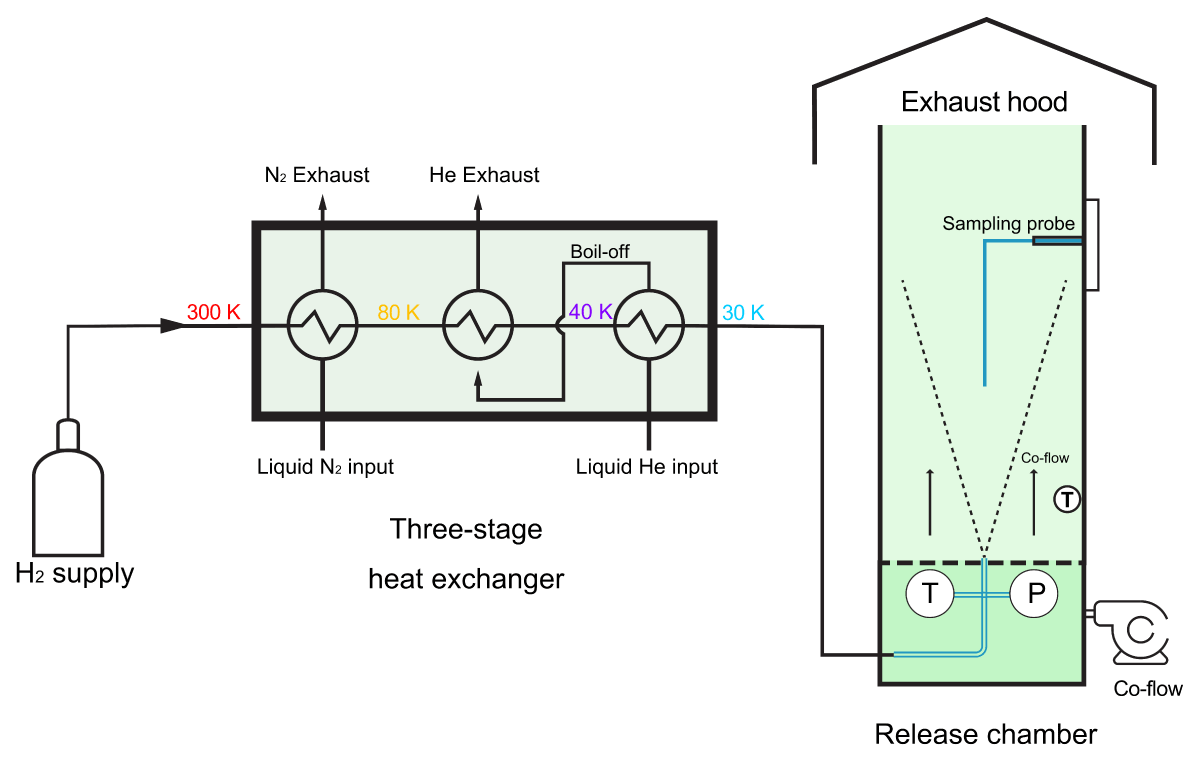
Figure 2
Schematic of the hydrogen release facility.
Table 2
Storage conditions for the release temperature test at fixed release pressure.
| TEST # | NOMINAL RELEASE PRESSURE (kPa) | p (kPa) | T (K) | D (mm) | Deff (mm) | JET REYNOLDS NUMBER (Rr)* 105 | MEASURED MASS FLOW RATE (g/s) | CALCULATED MASS FLOW RATE (g/s)* |
|---|---|---|---|---|---|---|---|---|
| 1 | 300 | 294 | 35 | 1 | 1.02 | 4.15 | 0.43 | 0.46 |
| 4 | 294 | 48 | 1 | 1.02 | 2.54 | 0.36 | 0.38 | |
| 7 | 298 | 70 | 1 | 1.03 | 1.47 | 0.29 | 0.32 | |
| 12 | 301 | 119 | 1 | 1.03 | 0.70 | 0.21 | 0.24 | |
| 17 | 297 | 290 | 1 | 1.04 | 0.21 | 0.13 | 0.15 | |
| 6 | 500 | 484 | 69 | 1 | 1.13 | 2.47 | 0.48 | 0.52 |
| 9 | 506 | 103 | 1 | 1.14 | 1.46 | 0.40 | 0.44 | |
| 13 | 509 | 126 | 1 | 1.15 | 1.07 | 0.34 | 0.39 | |
| 15 | 498 | 289 | 1 | 1.18 | 0.37 | 0.22 | 0.25 |
* The calculated mass flow rate assumes choked flow using the nozzle diameter and upstream temperature and pressure of the nozzle. Same for Table 3.
Table 3
Storage conditions for the release temperature test at fixed mass flow rates.
| TEST # | NOMINAL MASS FLOW RATE (G/S) | P (KPA) | T (K) | D (MM) | DEFF (MM) | JET REYNOLDS NUMBER (RE)* 105) | MEASURED MASS FLOW RATE (G/S) | CALCULATED MASS FLOW RATE (G/S) |
|---|---|---|---|---|---|---|---|---|
| 7 | 0.30 | 298 | 70 | 1 | 1.03 | 1.47 | 0.29 | 0.32 |
| 11 | 409 | 108 | 1 | 1.09 | 1.08 | 0.3 | 0.35 | |
| 14 | 627 | 290 | 1 | 1.27 | 0.50 | 0.3 | 0.32 | |
| 4 | 0.36 | 294 | 48 | 1 | 1.02 | 2.54 | 0.36 | 0.38 |
| 10 | 468 | 105 | 1 | 1.12 | 1.31 | 0.36 | 0.4 | |
| 18 | 747 | 290 | 1 | 1.35 | 0.60 | 0.36 | 0.38 | |
| 1 | 0.43 | 294 | 35 | 1 | 1.02 | 4.15 | 0.43 | 0.46 |
| 8 | 561 | 101 | 1 | 1.17 | 1.63 | 0.44 | 0.49 | |
| 16 | 959 | 289 | 1 | 1.48 | 0.71 | 0.43 | 0.47 |
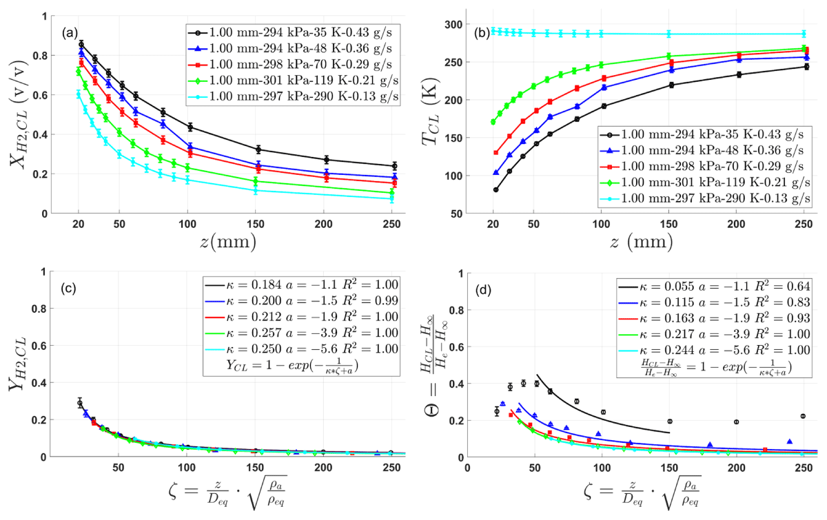
Figure 3
Centreline decay at the release temperature of 35–290 K and a fixed release pressure of 300 kPa: (a) hydrogen mole fraction, (b) mixture temperature, (c) hydrogen mass fraction decay correlation and (d) normalized mixture enthalpy decay correlation.
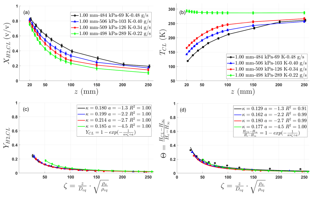
Figure 4
Centreline decay at the release temperature of 69–289 K and a fixed release pressure of 500 kPa: (a) hydrogen mole fraction, (b) mixture temperature, (c) hydrogen mass fraction decay correlation and (d) normalized mixture enthalpy decay correlation.
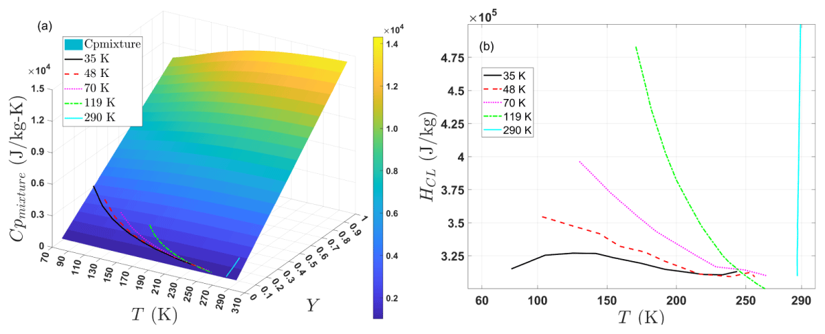
Figure 5
(a) Mixture mass-based Cp as a function of hydrogen mass fraction and mixture temperature. The lines represent the mixture Cp along the centreline for releases at 35–290 K; (b) centreline mixture enthalpy (HCL) as a function of mixture temperature for releases at 35–290 K.
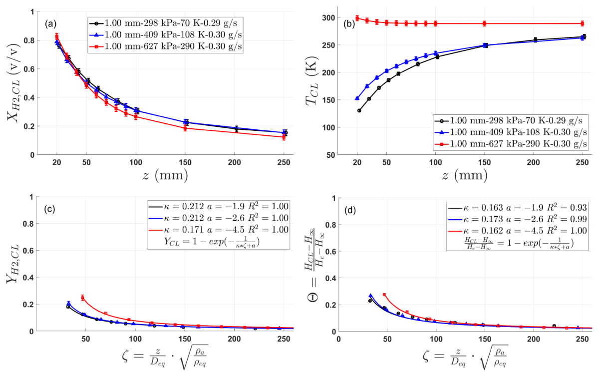
Figure 6
Centreline decay at the release temperature of 70–290 K and a fixed mass flow rate of 0.30 g/s: (a) hydrogen mole fraction, (b) mixture temperature, (c) hydrogen mass fraction decay correlation and (d) normalized mixture enthalpy decay correlation.
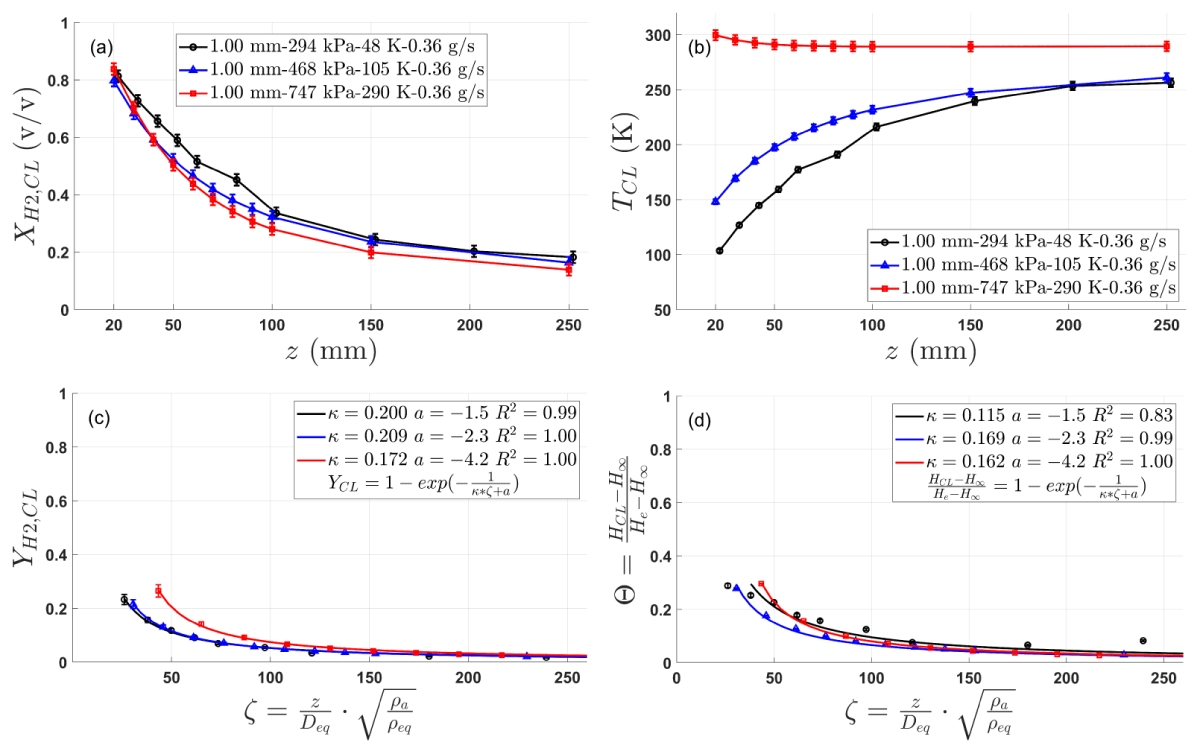
Figure 7
Centreline decay at the release temperature of 48–290 K and a fixed mass flow rate of 0.36 g/s: (a) hydrogen mole fraction, (b) mixture temperature, (c) hydrogen mass fraction decay correlation and (d) normalized mixture enthalpy decay correlation.
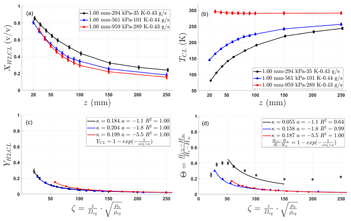
Figure 8
Centreline decay at the release temperature of 35–289 K and a fixed mass flow rate of 0.43 g/s: (a) hydrogen mole fraction, (b) mixture temperature, (c) hydrogen mass fraction decay correlation and (d) normalized mixture enthalpy decay correlation.
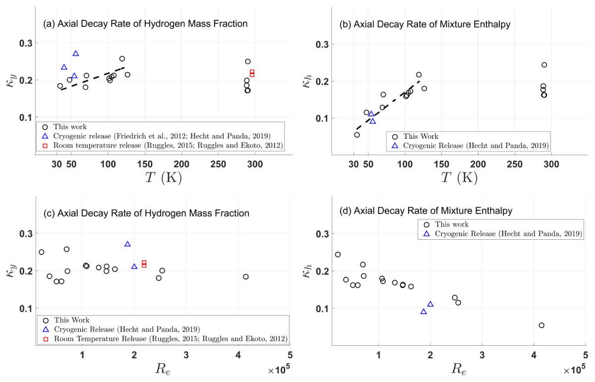
Figure 9
Centreline decay rate of mass fraction and enthalpy as a function of release temperature (a, b) and jet Reynolds number (c, d). Experimental data from this work (black circles), cryogenic literature data (blue triangles) (Friedrich et al., 2012; Hecht and Panda, 2019), room temperature literature data (red squares) (Ruggles, 2015; Ruggles and Ekoto, 2012). The dashed line in (a) and (b) indicates the trend of decay rate for the cryogenic jets measured in this work.
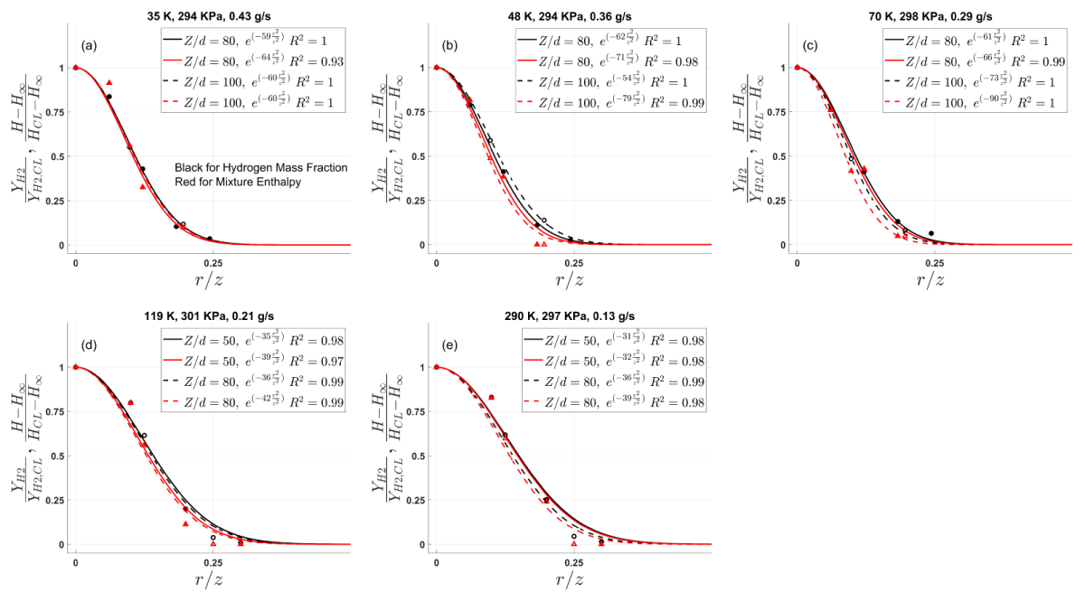
Figure 10
Radial decay of hydrogen mass fraction and mixture enthalpy at different release temperatures and a fixed release pressure of 300 kPa. (a) 35 K, (b) 48 K, (c) 70 K, (d) 119 K and (e) 297 K; black markers and lines represent normalized mass fraction, and red markers and lines represent normalized mixture enthalpy; different line types signify different downstream locations.
Table 4
Table for all radial decay Gaussian coefficients.
| TEST # | RELEASE TEMPERATURE (K) | RELEASE PRESSURE (KPA) | RELEASE MASS FLOW RATE (G/S) | MASS FRACTION ηY | ENTHALPY DECAY ηY | ||||||
|---|---|---|---|---|---|---|---|---|---|---|---|
| DOWNSTREAM LOCATION OF MEASUREMENTS (MM) | |||||||||||
| 50 | 80 | 90 | 100 | 50 | 80 | 90 | 100 | ||||
| Fixed pressure 300 KPa | |||||||||||
| 1 | 35 | 294 | 0.43 | 59 | 60 | 64 | 60 | ||||
| 4 | 48 | 294 | 0.36 | 62 | 54 | 71 | 79 | ||||
| 7 | 70 | 298 | 0.29 | 61 | 73 | 66 | 90 | ||||
| 12 | 119 | 301 | 0.21 | 35 | 36 | 39 | 42 | ||||
| 17 | 290 | 297 | 0.13 | 31 | 36 | 32 | 39 | ||||
| Fixed pressure 500 KPa | |||||||||||
| 6 | 69 | 484 | 0.48 | 38 | 34 | 38 | 38 | ||||
| 9 | 103 | 506 | 0.40 | 39 | 42 | 40 | 43 | ||||
| 13 | 126 | 509 | 0.34 | 22 | 18 | 23 | 22 | ||||
| 15 | 289 | 498 | 0.22 | 48 | 46 | 50 | 49 | ||||
| Fixed mass flow rate of 0.30 g/s | |||||||||||
| 7 | 70 | 298 | 0.29 | 61 | 73 | 66 | 90 | ||||
| 11 | 108 | 409 | 0.30 | 40 | 42 | 40 | 44 | 50 | 50 | ||
| 14 | 290 | 627 | 0.30 | 37 | 40 | 37 | 38 | 38 | 41 | 38 | 39 |
| Fixed mass flow rate of 0.36 g/s | |||||||||||
| 4 | 48 | 294 | 0.36 | 62 | 54 | 71 | 79 | ||||
| 10 | 105 | 468 | 0.36 | 44 | 46 | 45 | 49 | 54 | 57 | ||
| 18 | 290 | 747 | 0.36 | 37 | 38 | 35 | 36 | 38 | 39 | 36 | 37 |
| Fixed mass flow rate of 0.43 g/s | |||||||||||
| 1 | 35 | 294 | 0.43 | 59 | 60 | 64 | 60 | ||||
| 8 | 101 | 561 | 0.44 | 37 | 38 | 35 | 40 | 47 | 42 | ||
| 16 | 289 | 959 | 0.43 | 44 | 43 | 41 | 46 | 43 | 42 | ||
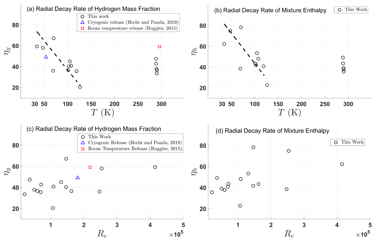
Figure 11
Radial decay rate of mass fraction and enthalpy as a function of release temperature (a, b) and jet Reynolds number (c, d). Experimental data from this work (black circles), cryogenic literature data (blue triangles) (Hecht and Panda, 2019), room temperature literature data (red squares) (Ruggles, 2015). The dashed line in (a) and (b) indicates the trend of decay rate for the cryogenic jets measured in this work.
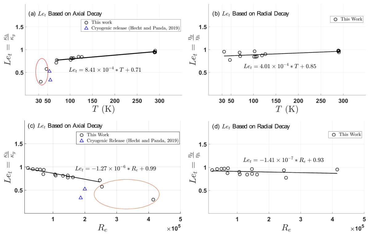
Figure 12
Let as a function of the release temperature, based on (a) the ratio of axial decay rates for enthalpy and mass fraction, and (b) the ratio of radial decay rates for mass fraction and enthalpy. The Let fitting for release temperature at 70 K or higher (35 and 50 K neglected and circled in red). Same Let plotted as a function of jet Reynolds number in (c) and (d). Experiment data from this work (black circle), literature data (blue triangle) (Hecht and Panda, 2019).
Table 5
Turbulent Prt and Sct estimation for release at 103 K, 506 KPa.
| PARAMETERS | VALUE | |
|---|---|---|
| Axial decay rate | Mass fraction κy | 0.199 (measured) |
| Enthalpy κh | 0.162 (measured) | |
| Velocity κv | 0.156 (CFD) | |
| Axial turbulent parameters | 0.81 (measured) | |
| 0.96 (calculated using CFD) | ||
| 0.78 (calculated using CFD) | ||
| Radial decay rate | Mass fraction ηy | 40.5 (measured) |
| Enthalpy ηh | 41.5 (measured) | |
| Velocity ηv | 62 (CFD) | |
| Radial turbulent parameters | 0.96 (measured) | |
| 0.67 (calculated using CFD) | ||
| 0.65 (calculated using CFD) | ||
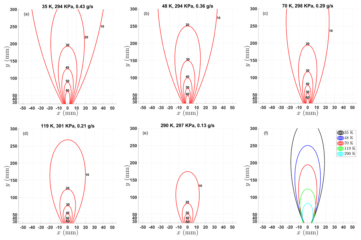
Figure 13
Hydrogen mole fraction (%) contour at different release temperatures and a fixed release pressure of 300 KPa: (a) 35 K, (b) 48 K, (c) 70 K, (d) 119 K, (e) 290 K and (f) contours of 20% H2 mole fraction at different release temperatures.
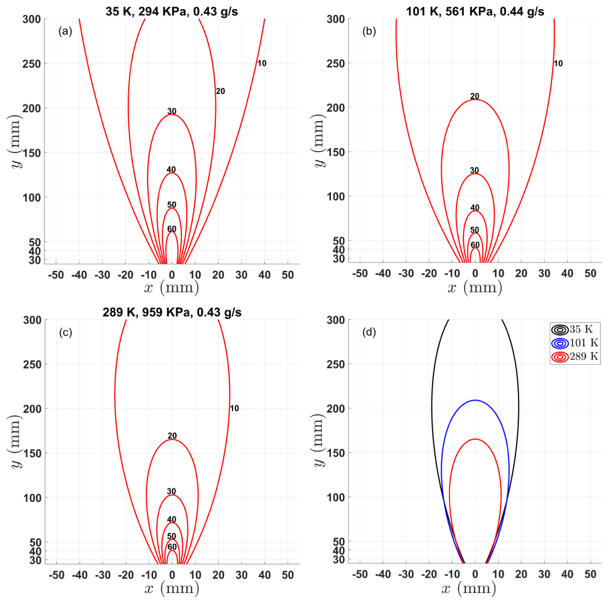
Figure 14
Hydrogen concentration contour at different release temperatures and a fixed mass flow rate of 0.43 g/s: (a) 35 K, (b) 101 K, (c) 289 K and (d) contours of 20% H2 mole fraction at different release temperatures.
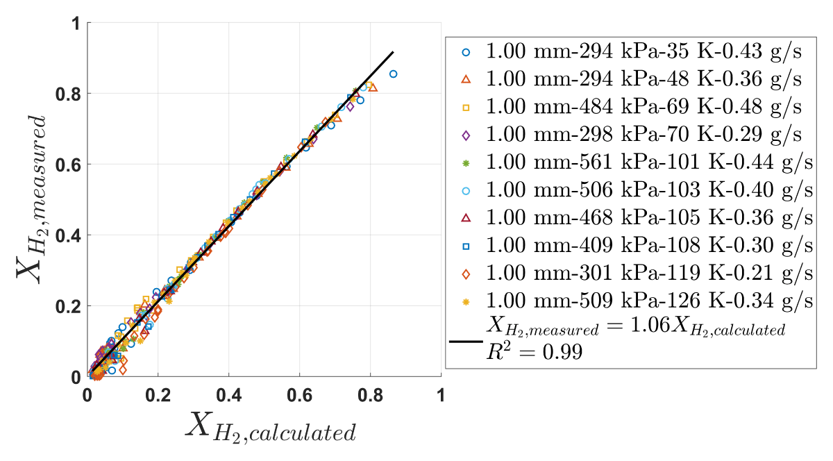
Figure 15
Examination of the applicability of adiabatic mixing to the cryogenic release experiments. XH2,calculated is from equation (7). Both axial and radial measurements are plotted; the black line is the linear fitting of all plotted data. A slope of 1 means perfect adiabatic mixing.
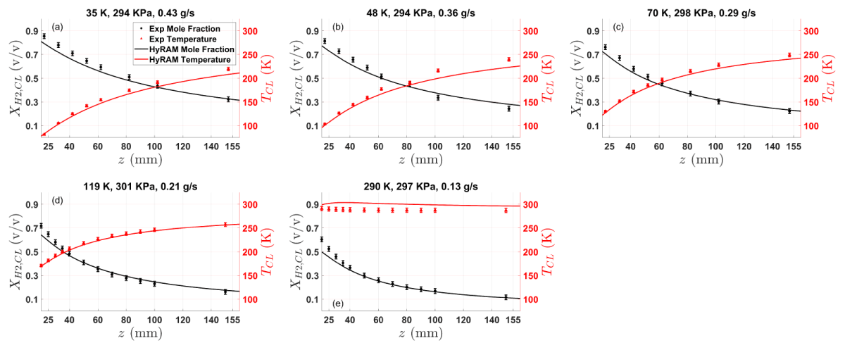
Figure 16
Comparison of measured and simulated centreline hydrogen molar fraction and mixture temperature at different release temperatures and a fixed release pressure of 300 kPa: (a) 35 K, (b) 48 K, (c) 70 K, (d) 119 K and (e) 290 K; symbols for experiment data and curves for HyRAM simulation; black for hydrogen mole fraction and red for mixture temperature.
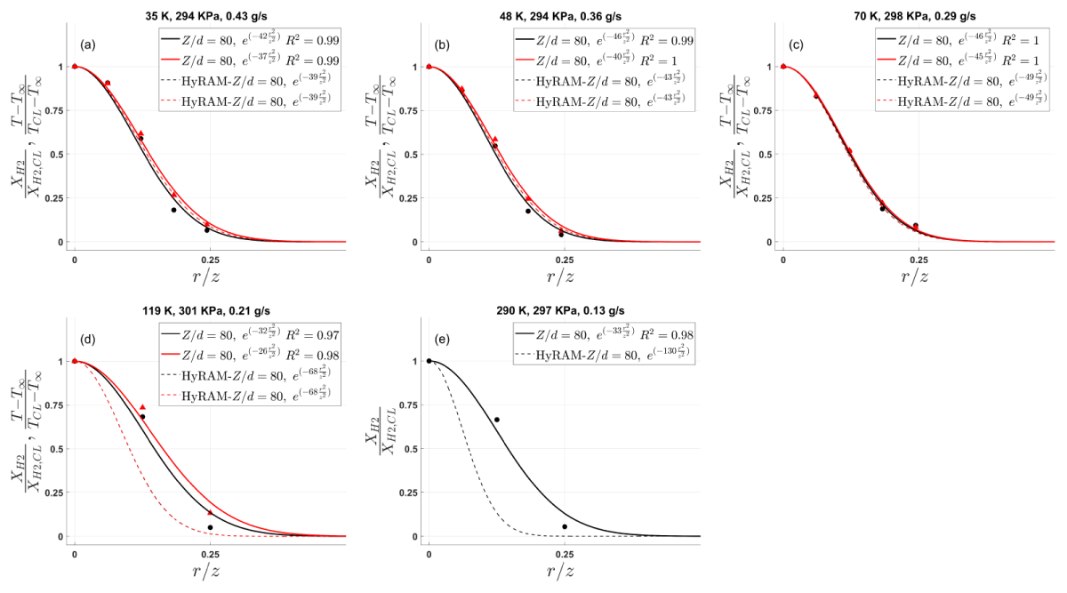
Figure 17
Comparison of the measured and simulated radial hydrogen mole fraction and mixture temperature at different release temperatures and a fixed release pressure of 300 kPa, (a) 35 K, (b) 48 K, (c) 70 K, (d) 119 K and (e) 290 K; solid lines are fitted from measurements (markers) and dashed lines represent results from the HyRAM+ 6.0 simulation; black for hydrogen mole fraction and red for mixture temperature.