
Nomenclature
Latin Symbols
- a
offset in hyperbolic relations
- Cp
mass-based specific heat
molar-based specific heat
- D
nozzle diameter
- H
enthalpy
- T
temperature
- v
velocity
- Y
mass fraction
- r
radial distance
- z
axial distance
- Le
Lewis number
- Pr
Prandtl number
- Sc
Schmidt number
- Re
Reynolds number
Greek Symbols
- κ
axial decay rate
- η
radial decay rate
- ρ
density
Subscripts
- a
ambient air
- ∞
ambient
- cl
centreline
- e
nozzle exit
- eq
equivalent of notional nozzle exit
- eff
effective
- h
enthalpy
- mix
mixture
- r
storage
- t
turbulent
- v
velocity
- y
mass fraction
1. Introduction
Hydrogen is attracting major interest as a clean energy carrier and carbon-free fuel. To overcome the low volumetric energy density, hydrogen is commonly stored as a liquid or as a high-pressure gas. The former offers higher density and thus is more suitable for long-distance transport (Yue et al., 2021). Leaks of liquid hydrogen, however, produce high-density, highly flammable mixtures which pose major fire and explosion risks to the surroundings (LaChance et al., 2009; Schefer et al., 2011). An accurate understanding of cryogenic hydrogen dispersion behaviours is therefore essential for LH2 handling, storage and transport (NFPA, 2023).
In the following, we firstly review the general characteristics of underexpanded jets and classic methods for analysis of decay rates, then review existing hydrogen release experiments in laboratory settings in the form of both high-pressure gases and cryogenic fluids, and finally present the objective of this work.
1.1 Characteristics of free jet mixing into still air
Liquid hydrogen can be released as a multi-phase jet or a vapour-only jet. The vapour-only release, typically involved in small leaks, can be characterized by an underexpanded jet, choked at the leak point (Courant and Friedrichs, 1948; Shapiro, 1953). The underexpanded region contains complex shock structures which are typically influenced by the exit geometry and the pressure ratio between the storage and the ambient (Franquet et al., 2015). The intricate interactions of shocks are not essential for the subsequent jet development and are often modelled with notional nozzles that transform the exit flow into a subsonic jet with an equivalent diameter (Birch et al., 1984; Birch et al., 1987; Ewan and Moodie, 1986; Molkov, 2012; Yuceil and Otugen, 2002). The downstream dispersion can then be characterized by a subsonic, turbulent, free jet that exhibits self-similar features as depicted in Figure 1 and analysed below.
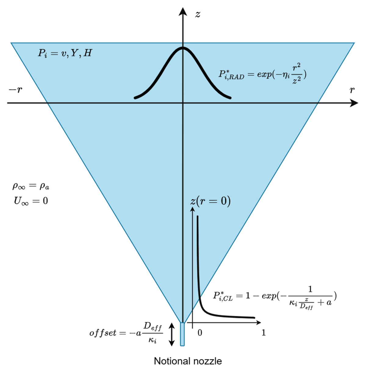
Figure 1
Schematic of scalar dissipation in an ideally expanded jet issued from a notional nozzle. Scalar decay can be described by a hyperbolic function along the axial direction and a Gaussian function along the radial direction (Kleinstein, 1964).
Kleinstein (1964) proposed a method for analysing turbulent, axisymmetric jets by linearization of the governing equations in the von Mise plane, coupled with an eddy viscosity formulation by Ferri, Libby, and Zakkay (1964). The axial decay is represented by a hyperbolic relationship between the decay parameter and the downstream distance, as shown in equation (1) for velocity, mass fraction and mixture enthalpy
where vcl and ve are the centreline and exit velocity, Ycl is the centreline mass fraction and Hcl, He and H∞ are the centreline, exit and ambient enthalpy, respectively. The decay rates are represented by κ, in which subscripts v, y, h refer to velocity, mass fraction and enthalpy, respectively. z is the downstream distance, a is the offset for the virtual origin and Deff is the effective diameter, defined as , where Deq and ρeq are the equivalent diameter and jet density at the exit of the notional nozzle model, and ρa is the ambient air density.
In the far field, this hyperbolic relationship can be reduced to a linear function between the inverse of the scalar and normalized distance (Chen and Rodi, 1980; So and Aksoy, 1993), as shown in equation (2).
All hydrogen release experiments to date have adopted this expression for decay analysis, although the definition of effective diameter was somewhat different among the studies, as summarized in Table 1. Nevertheless, the approximation to equation (1) is only valid for far downstream locations, and errors have been reported for using this formulation in near-nozzle regions (Li et al., 2018; Okabayashi et al., 2019; Takeno et al., 2017).
Table 1
Release conditions, measurement methods and centreline decay rates of past hydrogen release experiments.
| EXPERIMENT | RELEASE TEMPERATURE AND PRESSURE | NOZZLE DIAMETER (MM) | MEASURED PARAMETER (P) | MEASUREMENT METHOD | EFFECTIVE NOZZLE SIZE (DEFF) | CENTRELINE DECAY RATE (P*–1 VS. Z/DEFF) (EQUATION (2)) |
|---|---|---|---|---|---|---|
| Friedrich et al. (2012) | 34–65 K 7–35 bar | 0.5, 1 | Mass fraction | BOS and thermal couples | 0.233 | |
| Hecht and Panda (2019) | 48–61 K 2–5 bar | 1, 1.25 | Mass fraction, mixture temperature | Raman scattering | 0.277 (mass) 0.0281 (temp) | |
reanalysis with noise reduction (Li et al., 2023) | 0.22 (mass) 0.023 (temp) | |||||
| Veser et al. (2011)* | 35, 80 and 290 K 5–60 bar | 1, 2, 4 | Velocity, mass fraction | PIV and Sampling probe** | 0.193 (velocity) 0.313 (mass) | |
| Ruggles, (2015) and Ruggles and Ekoto (2012) | 296 K 10 bar | 1.5 | Mass fraction | Rayleigh scattering | 0.214 (Ruggles, 2015) 0.222 (Ruggles and Ekoto, 2012) | |
| Ruffin, Mouilleau and Chaineaux (1996)* | 288 K 40 bar | 25 | Mass fraction | Pellistor hydrogen sensor | 0.27 |
P: measured scalar; P*: normalized scalar, definition in equation (2); Deq: equivalent diameter (notional nozzle exit); De: nozzle diameter; ρe: density at the nozzle exit; ρeq: equivalent density at notional nozzle exit; ρa: ambient air density; ρr: storage density.
*Horizontal release.
**Hydrogen analysed offline, sensor type not reported.
From the obtained decay rates, dimensionless parameters for turbulent mixing can be derived (Kleinstein, 1964), as shown in equation (3).
The turbulent parameters can be derived from ratios between different κ. Specifically, Prt represents the relative decay rate of velocity and enthalpy, Sct the ratio between velocity and mass fraction and Let the ratio between enthalpy and mass fraction decay rates (Kleinstein, 1964). Two out of the three are required to define the system.
On the radial direction, the scalar decay is described by a Gaussian distribution (equation (4))
where the decay rates are represented by the Gaussian coefficient η, and r is the radial distance (Corrsin and Uberoi, 1949; Chen and Rodi, 1980; Kleinstein, 1964). Kleinstein’s analysis yielded a comparable expression to the same effect. Similarly, turbulent mixing parameters can be derived for the radial direction from η (equation (5))
1.2 Compressed room-temperature hydrogen jet mixing in still air
Hydrogen releases at room temperature have been reported by Ruggles and Ekoto (2012) at Sandia. They conducted vertical releases at stagnation conditions of 9.83 bar and 296 K through a 1.5-mm diameter orifice. Rayleigh scattering was used to obtain the mole fraction of hydrogen. The centreline mass fraction decay rate was determined to be 0.214 with static air and 0.222 with 0.5 m/s co-flow air (Ruggles, 2015). The experiment also measured radial mass fraction data, and by normalizing with the centreline value, all radial mass fraction distributions were characterized by a single Gaussian function with a coefficient η of 59. This value matched an earlier study of helium, methane and propane releases at room temperature (Richards and Pitts, 1993).
Horizontal room temperature releases were reported by Ruffin, Mouilleau and Chaineaux (1996) at 40 bar with 25–100 mm nozzles. The centreline mass fraction decay rate was found to be 0.27, with the downstream distance normalized by the notional nozzle equivalent exit diameter and density (Birch et al., 1984). Other horizontal room-temperature releases reported the centreline mass fraction decay rates around 0.3 (Okabayashi et al., 2019; Takeno et al., 2017), which are higher than those from vertical experiments, but similar to those from cryogenic horizontal releases by Veser et al. (2011).
1.3 Cryogenic hydrogen jet mixing in still air
Friedrich et al. (2012) from Karlsruhe Institute of Technology conducted vertical hydrogen releases at temperatures from 34 to 65 K and pressures from 7 to 35 bar using 0.5 and 1 mm nozzles. The lowest measurement is 40 mm above the release point. Background Oriented Schlieren (BOS) technique was used to determine the density gradient. The centreline hydrogen concentration was calculated using the density gradient and temperature measurement (with thermocouples) at different downstream locations. The centreline mass fraction decay rate was obtained from the concentration profiles to be 0.233 using equation (2), where the effective nozzle diameter was obtained using the exit diameter and hydrogen storage density.
Hecht and Panda (2019) conducted vertical cryogenic hydrogen releases at Sandia National Laboratory with the release condition of 48 to 63 K and 2–5 bar using 1 and 1.25 mm nozzles. Their work reported the only set of data for concentration and temperature along both axial and radial directions. Raman scattering was used to determine the hydrogen and nitrogen (air) concentrations using two cameras, where the gas temperature was calculated using the ideal gas law. The lowest measurement is 38 mm above the release point. Based on their published data, the measurement uncertainty is estimated to be ±5 mol% for hydrogen from 40 to 80 mol% and ±20 K for temperature from 100 to 210 K. The axial mass fraction decay rate was reported to be 0.277, where the downstream distance is normalized with the exit diameter and hydrogen storage density. The axial decay rate for the normalized temperature is nearly one order of magnitude smaller, 0.0281. In the radial direction, the mass fraction and temperature both follow a Gaussian distribution (equation (4)), and a single Gaussian coefficient can describe the decay of a given scalar at different axial locations, for example, η = 49 and 42 for hydrogen mass fraction and mixture temperature, respectively. A later paper reanalysed the Raman results (Li et al., 2023) by reducing the measurement noise and reported lower axial decay rates, 0.22 and 0.023 for mass fraction and temperature, respectively. The Gaussian coefficient for the radial temperature profile was also updated to be 50, whereas that for the radial mass fraction profile remained as 49. These updated decay rates matched more closely with hydrogen mass fraction results from previous room-temperature release experiments (Richards and Pitts, 1993; Ruggles, 2015) reviewed above.
Veser et al. (2011) conducted horizontal cryogenic hydrogen releases with storage pressures of 8.25–68.5 bar and release temperatures of 35, 80 and 290 K using round nozzles of 1, 2 and 4 mm diameter at Forschungszentrum Karlsruhe (FZK) facilities. They found buoyancy playing a significant role in the axial decay of velocity and hydrogen concentration and reported a larger centreline mass fraction decay rate (0.313) than those with vertical release.
A summary of laboratory hydrogen release experiments reviewed is provided in Table 1.
CFD and low-order models have been used to simulate these experiments. A common assumption in the CFD simulations is the turbulent Prandtl number (Prt) and Schmidt number (Sct) being equal (Giannissi and Venetsanos, 2018; Giannissi et al., 2021; Saini et al., 2024), which by definition set the turbulent Lewis number (Let) to unity. Kleinstein (1964) applied equation (4) to room-temperature helium/air jets and yielded a Prt of 0.715 and Sct of 0.708, giving a Let of 0.99. Similar studies for hydrogen/air jets or cryogenic jets have not been reported.
1.4 Objective of this work
Cryogenic hydrogen can be released at a temperature well below that for air condensation, which significantly alters the thermodynamic and transport properties of involved gases, affects the heat/mass transfer and subsequently impacts the jet dispersion (Hu et al., 2023; Matheis et al., 2020; Traxinger Banholzer and Pfitzner, 2018). From the review above, a systematic investigation of the impact of release temperature on hydrogen dispersions has not been reported. Among the few experiments for cryogenic hydrogen release, most have reported only the concentration in the axial direction where the measurements bear significant uncertainties from the optical methods used (Friedrich et al., 2012; Hecht and Panda, 2019). The impact of release temperature has been studied only by comparing data from different experiments, limiting the accuracy of the comparison.
To address this gap, this work conducts independent hydrogen concentration and mixture temperature measurements for both cryogenic and room-temperature releases in a single experimental setup. We use a movable sampling probe with two degrees of freedom to measure the decay of hydrogen mass fraction and enthalpy along both the axial and radial directions over a wide range of release temperatures, pressures, and mass flow rates. These decay rates are compared with data from the literature as well as simulation results using a low-order model, HyRAM+ 6.0 (Ehrhart et al., 2025). The treatment of Kleinstein (1964) is adopted to derive turbulent transport parameters, from which the impact of release temperature on hydrogen jet mixing is elucidated.
2. Methodology
2.1 Cryogenic release facility
Figure 2 shows a schematic of the hydrogen release facility at the University of Melbourne. The main components include a cryogenic heat exchanger and a release chamber. The heat exchanger uses three-stage cooling, a similar design to that in the Sandia experiment (Hecht and Panda, 2019; Panda and Hecht, 2017). The first stage uses a liquid nitrogen bath to cool the room temperature hydrogen (in coil flow) to around 80 K. The second stage is a counter-flow heat exchanger which uses the boil-off helium from the third stage to cool hydrogen to approximately 40 K. The third stage uses a liquid helium bath to cool the hydrogen further down to approximately 30 K. The temperatures at the inlets of the first and second stages and the outlet of the third stage are monitored using silicon diodes (Lakeshore DT-670). Liquid hydrogen and liquid helium are supplied from the respective dewars with the liquid level monitored with level sensors. The system is designed for a hydrogen flow rate up to 1 g/s and an operating pressure up to 10 bar.
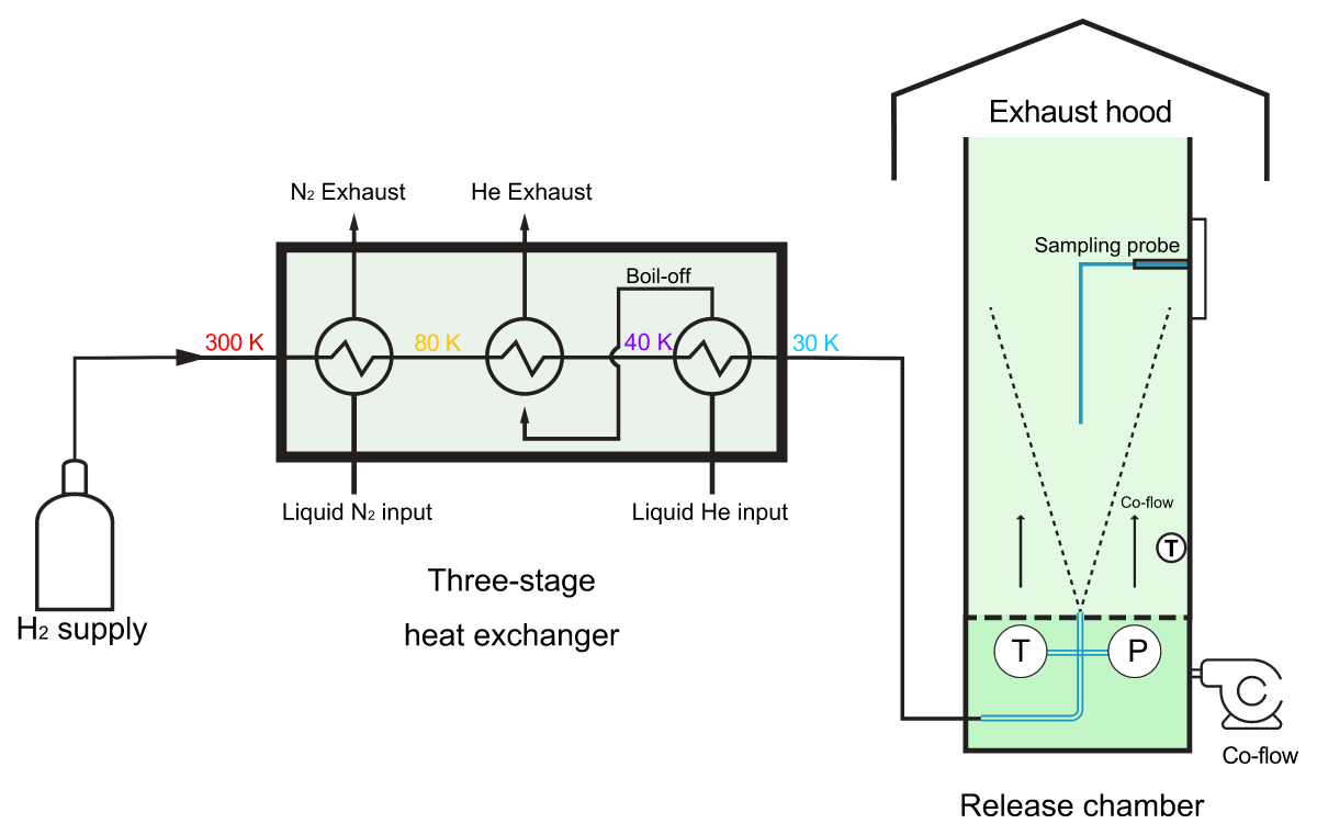
Figure 2
Schematic of the hydrogen release facility.
A vacuum-jacketed transfer hose connects the heat exchanger outlet to the release chamber. The hose is fitted with a silicon diode temperature sensor (Lakeshore DT-670) and a pressure transducer (Omega PXM519-010BAS2IS), which is installed at 68 mm upstream of the release orifice to indicate the storage temperature and pressure. Round-shaped orifices of 0.75, 1 and 1.25 mm diameter are used. The orifice was drilled into a stainless steel plate of 20 mm diameter and 0.73 mm thickness bolted to the end of the transfer hose.
The release chamber has a cross-section of 0.5 m by 0.5 m and a height of 2.5 m. The orifice is located at the centre of the base plane. Air co-flow is supplied from the bottom through a honeycomb panel (flush with the orifice exit) to provide a consistent chamber environment for different release conditions. To circumvent icing from air moisture, dry air is used for all releases reported here (cryogenic and room-temperature). The air is supplied from a 50-bar compressor with a refrigeration dryer at a flow rate of 30 g/s, giving an average co-flow velocity of 0.1 m/s. The relative humidity of the co-flow is 5–7%, measured using a humidity sensor underneath the honeycomb. The hydrogen/air mixture is extracted via a fume hood (0.9 m by 0.9 m) above the release chamber, which dilutes the mixture below the lower flammability limit (4 vol%) before entering the lab exhaust system. Thermocouples are installed inside the chamber to detect any ignition event, which will shut down the hydrogen flow and trigger an emergency response.
A sampling probe is installed inside the release chamber to measure hydrogen mole fraction and gas temperature. The probe is made of an ultra-low thermal conductivity material, G10, with a 3-mm inner diameter and 1-mm thickness. The probe is installed on a linear traverse platform (Zaber X-LRT-EC) with two degrees of freedom. From the release point, the probe can move from 20-1500mm along the vertical direction and 0–50 mm along the horizontal direction. The temperature is measured with a silicon diode sensor (Lakeshore DT-670) installed inside the G10 tube flush with the probe inlet. The hydrogen mole fraction is measured with a thermal conductivity detector (XEN-5320-HP-USB) installed approximately 800 mm away from the probe inlet. A gas sample is pulled past the sensor and through the tube by a small vacuum generator mounted on the stage of the linear traverse. This vacuum generator is based on the Venturi effect and operated with a small air flow. The analyser has an absolute uncertainty of ±2 vol% and a response time of less than one second. The silicon diode sensor has an uncertainty of ±0.5 K between 2 and 305 K. Measurement and control are realized via an in-house LabVIEW program.
For each release, Schlieren imaging is employed at the beginning to check the verticality of the released jet. After this is verified, a ‘symmetry test’ is conducted, which measures the hydrogen mole fraction and temperature at symmetrical radial positions and 20, 30 and 40 mm above the nozzle, to ensure that the probe is positioned at the centre of the jet.
The presence of the sampling probe can induce bias in the concentration and temperature measurements. Existing literature suggests limited impact on the upstream velocity (within 1–2 probe diameters) (Olshefski et al., 2022; Schlichting and Gersten, 2017) and a small bias on composition measurements (Bilger and Beck, 1975; Kent and Bilger, 1973; Lupant, Pesenti, and Lybaert, 2010). This probe-induced bias is assumed to be covered in the H2 sensor’s stated absolute uncertainty (±2%) in this work, which is subject to further investigations.
2.2 Release conditions
Two sets of experiments are conducted to investigate the effect of release temperature on hydrogen dispersion. The first uses constant storage pressure, which sets the pressure ratio and jet velocity, the most important parameters affecting the underexpanded jet in the near field. Storage pressures at approximately 3 and 5 bar are investigated. The second set uses a constant mass flow rate (0.30, 0.36, 0.43 g/s), which sets the jet Reynolds number, the primary parameter controlling the jet decay and turbulent mixing. Due to the significant variation in hydrogen’s viscosity at cryogenic temperatures, the Reynolds number decreases with the storage temperature. Tables 2 and 3 list the conditions for the temperature sweep at fixed pressures and fixed mass flow rates, respectively. The mass flow rates of hydrogen were measured using a Coriolis flowmeter before the heat exchanger. Also reported is the calculated mass flow rate for choked flow using the storage conditions and thermodynamic properties from the REFPROP database (Lemmon, Huber and McLinden, 2013). The discrepancy between the two flow rates can be attributed to the discharge coefficient, as well as the uncertainty in measuring the storage temperature, pressure and orifice diameter. A similar discrepancy was also reported in Panda and Hecht (2017). Additional release cases not falling into these two sets are reported in the Supplementary Materials.
Table 2
Storage conditions for the release temperature test at fixed release pressure.
| TEST # | NOMINAL RELEASE PRESSURE (kPa) | p (kPa) | T (K) | D (mm) | Deff (mm) | JET REYNOLDS NUMBER (Rr)* 105 | MEASURED MASS FLOW RATE (g/s) | CALCULATED MASS FLOW RATE (g/s)* |
|---|---|---|---|---|---|---|---|---|
| 1 | 300 | 294 | 35 | 1 | 1.02 | 4.15 | 0.43 | 0.46 |
| 4 | 294 | 48 | 1 | 1.02 | 2.54 | 0.36 | 0.38 | |
| 7 | 298 | 70 | 1 | 1.03 | 1.47 | 0.29 | 0.32 | |
| 12 | 301 | 119 | 1 | 1.03 | 0.70 | 0.21 | 0.24 | |
| 17 | 297 | 290 | 1 | 1.04 | 0.21 | 0.13 | 0.15 | |
| 6 | 500 | 484 | 69 | 1 | 1.13 | 2.47 | 0.48 | 0.52 |
| 9 | 506 | 103 | 1 | 1.14 | 1.46 | 0.40 | 0.44 | |
| 13 | 509 | 126 | 1 | 1.15 | 1.07 | 0.34 | 0.39 | |
| 15 | 498 | 289 | 1 | 1.18 | 0.37 | 0.22 | 0.25 |
* The calculated mass flow rate assumes choked flow using the nozzle diameter and upstream temperature and pressure of the nozzle. Same for Table 3.
Table 3
Storage conditions for the release temperature test at fixed mass flow rates.
| TEST # | NOMINAL MASS FLOW RATE (G/S) | P (KPA) | T (K) | D (MM) | DEFF (MM) | JET REYNOLDS NUMBER (RE)* 105) | MEASURED MASS FLOW RATE (G/S) | CALCULATED MASS FLOW RATE (G/S) |
|---|---|---|---|---|---|---|---|---|
| 7 | 0.30 | 298 | 70 | 1 | 1.03 | 1.47 | 0.29 | 0.32 |
| 11 | 409 | 108 | 1 | 1.09 | 1.08 | 0.3 | 0.35 | |
| 14 | 627 | 290 | 1 | 1.27 | 0.50 | 0.3 | 0.32 | |
| 4 | 0.36 | 294 | 48 | 1 | 1.02 | 2.54 | 0.36 | 0.38 |
| 10 | 468 | 105 | 1 | 1.12 | 1.31 | 0.36 | 0.4 | |
| 18 | 747 | 290 | 1 | 1.35 | 0.60 | 0.36 | 0.38 | |
| 1 | 0.43 | 294 | 35 | 1 | 1.02 | 4.15 | 0.43 | 0.46 |
| 8 | 561 | 101 | 1 | 1.17 | 1.63 | 0.44 | 0.49 | |
| 16 | 959 | 289 | 1 | 1.48 | 0.71 | 0.43 | 0.47 |
The notional nozzle model by Yuceil and Otugen (2002) is used in this work. The model considers mass, momentum and energy conservation, as well as the atmospheric pressure at the nozzle exit. For the decay rate evaluation, the axial distance is normalized by as defined in equation (1).
3. Results and Discussion
3.1 Axial decay
3.1.1 Temperature sweep with fixed storage pressure
Figure 3 shows the centreline hydrogen molar fraction and mixture temperature as a function of axial distance at 300 kPa and 35–290 K. Both properties decrease rapidly near the nozzle and then approach a plateau with a gentler decay. Figure 4 shows the corresponding results at 500 kPa and 69–289 K. Error bars are included to account for sensor measurement uncertainties.
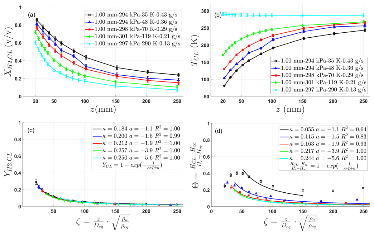
Figure 3
Centreline decay at the release temperature of 35–290 K and a fixed release pressure of 300 kPa: (a) hydrogen mole fraction, (b) mixture temperature, (c) hydrogen mass fraction decay correlation and (d) normalized mixture enthalpy decay correlation.
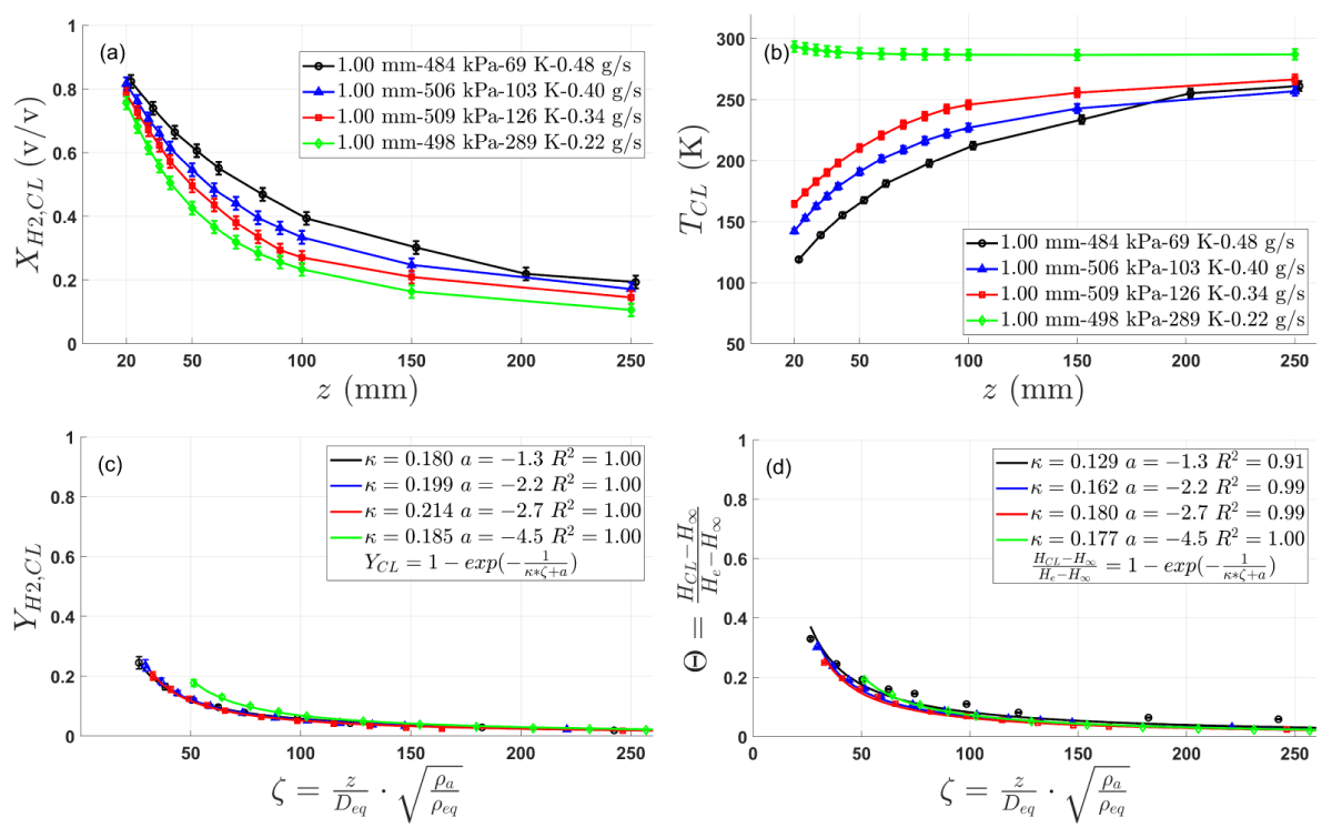
Figure 4
Centreline decay at the release temperature of 69–289 K and a fixed release pressure of 500 kPa: (a) hydrogen mole fraction, (b) mixture temperature, (c) hydrogen mass fraction decay correlation and (d) normalized mixture enthalpy decay correlation.
The hyperbolic decay of centreline mass fraction and normalized mixture enthalpy is shown in the subplots c and d in Figures 3 and 4. The hydrogen mass fraction correlates nearly perfectly with the normalized distance, as indicated by the R2 values. In the hyperbolic relation, κy represents the mass fraction decay rate in the axial direction. The virtual origin a is a fitted parameter and varies at each condition. The mass fraction decay rate ranges from 0.18 to 0.25, showing an increasing trend with release temperature (at both 300 and 500 kPa), although the trend is not preserved at room temperature. The decay rates fall into a similar range to those reported in previous studies (Table 1) calculated using the simplified correlation equation (2).
Correlation for the normalized mixture enthalpy decay uses the same offset as the corresponding mass fraction decay, assuming an equal origin for the mass and thermal mixing, as also used in Kleinstein’s study (1964). The hyperbolic correlation works excellently for cases above 50 K, where the enthalpy decay rate κh shows an increasing trend with the release temperature, similar to κy but with a consistently lower value. The correlation does work well for the 48 K case and not at all for the 35 K case, both at 300 kPa. This could be related to the non-monotonic variation of mixture enthalpy along the mixing process, as explained in the following.
Mixture enthalpy here is calculated using the measured gas temperature and mass fraction (equation (6)).
where Cp,H2 and Cp,air are the mass-based specific heat of pure H2 and air, respectively, at the mixture temperature (Tmix) from REFPROP (Lemmon, Huber and McLinden, 2013). The subscript mix refers to the mixture of hydrogen and air. Figure 5(a) shows the mixture Cp as a function of temperature and hydrogen fraction, with the 3-bar release cases at 35–290 K included as an example. Since the mass-based Cp of hydrogen is much larger than that of air, the mixture Cp decreases as the hydrogen concentration decreases, which occurs simultaneously as the mixture temperature increases. For the 35 and 50 K release cases, the net result is a non-monotonic variation of mixture enthalpy with temperature, as shown in Figure 5(b). This unusual behaviour causes a problem in analysing the enthalpy decay with Kleinstein’s method, which requires monotonic variation of the dimensionless flow properties, for example, those on the left-hand side of equation (1), from 1 (jet) to 0 (far field). While this is true for velocity and mass fraction, it is not the case for mixture enthalpy. For the 35 K release case, two local extreme values are noted, a maximum at 140 K and a minimum at 230 K, which challenges the application of the hyperbolic function to the problem.
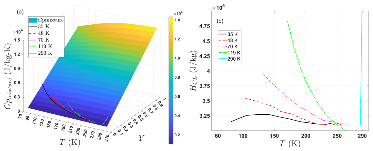
Figure 5
(a) Mixture mass-based Cp as a function of hydrogen mass fraction and mixture temperature. The lines represent the mixture Cp along the centreline for releases at 35–290 K; (b) centreline mixture enthalpy (HCL) as a function of mixture temperature for releases at 35–290 K.
One physical reason for the non-monotonicity of the coldest cases could be air condensation near the nozzle, which has been observed by Mie scattering in the 35 and 48 K cases (to be published in a future paper). The heat released from the phase change could alter the local mixture enthalpy, degrading the fit of the centreline decay equation (equation (1)).
3.1.2 Temperature sweep with fixed mass flow rate
Figures 6, 7, 8 show the centreline decay at constant mass flow rates of 0.30, 0.36 and 0.43 g/s with different release temperatures. The mass fraction decay is fitted excellently with Kleinstein’s method. The enthalpy decay also fits very well, except for the two deep cryogenic cases at 35 and 48 K discussed above. The increasing trend in κy and κh with release temperature is generally observed among the cryogenic cases, which is disrupted at room temperatures. Similar to the fixed pressure cases, the decay of enthalpy is slower than that of mass fraction along the centreline at corresponding conditions.
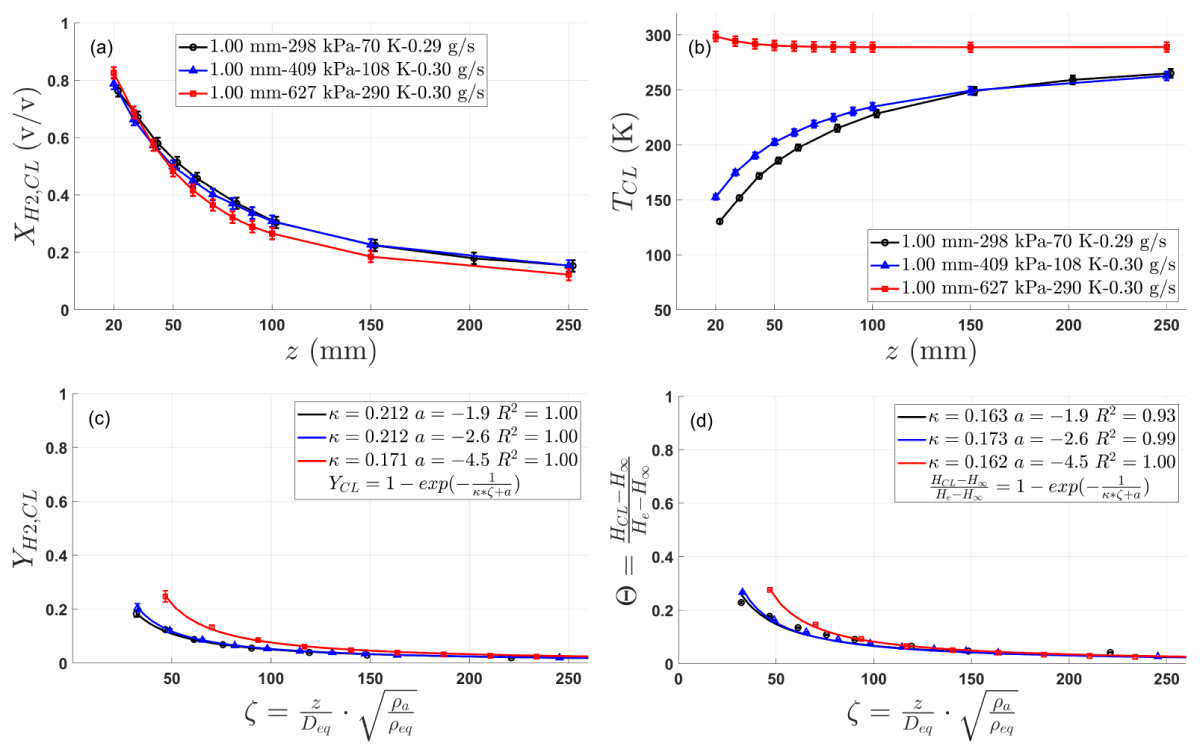
Figure 6
Centreline decay at the release temperature of 70–290 K and a fixed mass flow rate of 0.30 g/s: (a) hydrogen mole fraction, (b) mixture temperature, (c) hydrogen mass fraction decay correlation and (d) normalized mixture enthalpy decay correlation.
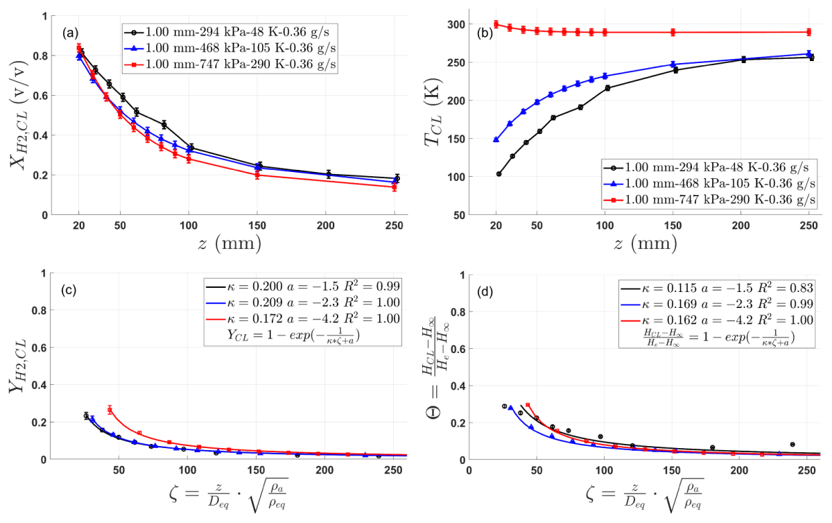
Figure 7
Centreline decay at the release temperature of 48–290 K and a fixed mass flow rate of 0.36 g/s: (a) hydrogen mole fraction, (b) mixture temperature, (c) hydrogen mass fraction decay correlation and (d) normalized mixture enthalpy decay correlation.
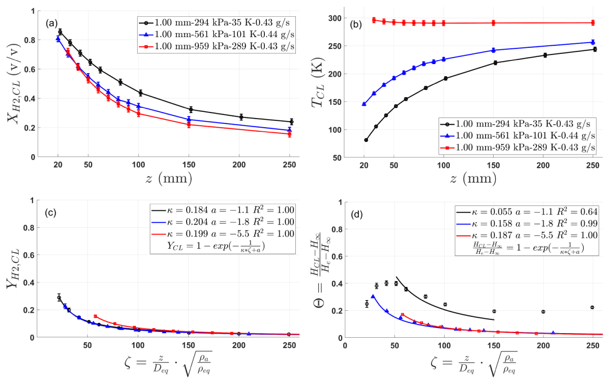
Figure 8
Centreline decay at the release temperature of 35–289 K and a fixed mass flow rate of 0.43 g/s: (a) hydrogen mole fraction, (b) mixture temperature, (c) hydrogen mass fraction decay correlation and (d) normalized mixture enthalpy decay correlation.
To evaluate the parameters influencing the axial decay, κy and κh are plotted against release temperature for all data obtained in this work and those from the literature (Table 1). The dependence on jet Reynolds number is also plotted for comparison. Figure 9 shows that for the data measured in the current study, the mass fraction decay rate exhibits an apparent increasing trend with release temperature for cryogenic release cases (35–119 K), as well as a slightly decreasing trend with jet Reynolds number overall. These trends are more evident with the enthalpy decay rate. The dependence on jet Reynolds number seems counterintuitive but can be explained by the fact that the highest Re cases are those with the lowest release temperature. Both figures are therefore consistent and indicate that the release temperature is important in determining the scalar decay, in particular, a colder release temperature leading to slower mixing in the axial direction.
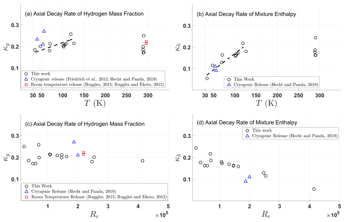
Figure 9
Centreline decay rate of mass fraction and enthalpy as a function of release temperature (a, b) and jet Reynolds number (c, d). Experimental data from this work (black circles), cryogenic literature data (blue triangles) (Friedrich et al., 2012; Hecht and Panda, 2019), room temperature literature data (red squares) (Ruggles, 2015; Ruggles and Ekoto, 2012). The dashed line in (a) and (b) indicates the trend of decay rate for the cryogenic jets measured in this work.
3.2 Radial decay
The radial distribution of hydrogen mass fraction and mixture enthalpy was measured at 50–100 mm above the nozzle. The measurements are considered in the self-similar region, where the scalar distribution follows the Gaussian function (Chen and Rodi, 1980; Hecht and Panda, 2019; Kleinstein, 1964; Ruggles, 2015). Figure 10 shows the Gaussian profiles for the release temperature sweep with a constant release pressure of 300 kPa, where the scalar is normalized by the centreline value, and the radial distance is normalized by the axial location where the measurement is conducted. Overall, a good fit is obtained for both the mass fraction and enthalpy dispersion. It is worth noting that for some release conditions, the minimum mixture enthalpy is not in the far field but closer to the jet, due to the non-monotonic variation discussed above. In these cases, the normalization uses the smallest enthalpy as H∞. This change had a minimal impact on the final Gaussian coefficients reported, as points further away from the centreline have a smaller weight on the fitting.
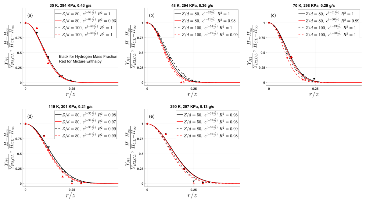
Figure 10
Radial decay of hydrogen mass fraction and mixture enthalpy at different release temperatures and a fixed release pressure of 300 kPa. (a) 35 K, (b) 48 K, (c) 70 K, (d) 119 K and (e) 297 K; black markers and lines represent normalized mass fraction, and red markers and lines represent normalized mixture enthalpy; different line types signify different downstream locations.
Table 4 summarises the radial decay rates for the temperature sweep at 300 and 500 kPa and those at fixed mass flow rates. The figures for the other conditions are reported in the Supplementary Materials. Within each dataset, the Gaussian coefficients do not show a clear dependence on the release temperature. On the other hand, the decay rates of mass fraction and enthalpy are similar in each case, but the former is consistently smaller by a small margin, except for the 35 K and 48 K cases.
Table 4
Table for all radial decay Gaussian coefficients.
| TEST # | RELEASE TEMPERATURE (K) | RELEASE PRESSURE (KPA) | RELEASE MASS FLOW RATE (G/S) | MASS FRACTION ηY | ENTHALPY DECAY ηY | ||||||
|---|---|---|---|---|---|---|---|---|---|---|---|
| DOWNSTREAM LOCATION OF MEASUREMENTS (MM) | |||||||||||
| 50 | 80 | 90 | 100 | 50 | 80 | 90 | 100 | ||||
| Fixed pressure 300 KPa | |||||||||||
| 1 | 35 | 294 | 0.43 | 59 | 60 | 64 | 60 | ||||
| 4 | 48 | 294 | 0.36 | 62 | 54 | 71 | 79 | ||||
| 7 | 70 | 298 | 0.29 | 61 | 73 | 66 | 90 | ||||
| 12 | 119 | 301 | 0.21 | 35 | 36 | 39 | 42 | ||||
| 17 | 290 | 297 | 0.13 | 31 | 36 | 32 | 39 | ||||
| Fixed pressure 500 KPa | |||||||||||
| 6 | 69 | 484 | 0.48 | 38 | 34 | 38 | 38 | ||||
| 9 | 103 | 506 | 0.40 | 39 | 42 | 40 | 43 | ||||
| 13 | 126 | 509 | 0.34 | 22 | 18 | 23 | 22 | ||||
| 15 | 289 | 498 | 0.22 | 48 | 46 | 50 | 49 | ||||
| Fixed mass flow rate of 0.30 g/s | |||||||||||
| 7 | 70 | 298 | 0.29 | 61 | 73 | 66 | 90 | ||||
| 11 | 108 | 409 | 0.30 | 40 | 42 | 40 | 44 | 50 | 50 | ||
| 14 | 290 | 627 | 0.30 | 37 | 40 | 37 | 38 | 38 | 41 | 38 | 39 |
| Fixed mass flow rate of 0.36 g/s | |||||||||||
| 4 | 48 | 294 | 0.36 | 62 | 54 | 71 | 79 | ||||
| 10 | 105 | 468 | 0.36 | 44 | 46 | 45 | 49 | 54 | 57 | ||
| 18 | 290 | 747 | 0.36 | 37 | 38 | 35 | 36 | 38 | 39 | 36 | 37 |
| Fixed mass flow rate of 0.43 g/s | |||||||||||
| 1 | 35 | 294 | 0.43 | 59 | 60 | 64 | 60 | ||||
| 8 | 101 | 561 | 0.44 | 37 | 38 | 35 | 40 | 47 | 42 | ||
| 16 | 289 | 959 | 0.43 | 44 | 43 | 41 | 46 | 43 | 42 | ||
Figure 11 plots the Gaussian coefficients as a function of release temperature and jet Reynolds number for all cases investigated. Additional data from the literature for mass fractions are also included.1 Among the cryogenic cases, an apparent decreasing trend with increasing release temperature is observed for both ηy and ηh, indicating faster mixing at decreased release temperature. However, the room temperature cases do not follow this trend. This is consistent with the axial results above, although significant scattering exists. On the Reynolds number scale, no clear trend can be identified, suggesting Reynolds number does not play a significant role in the radial decay.
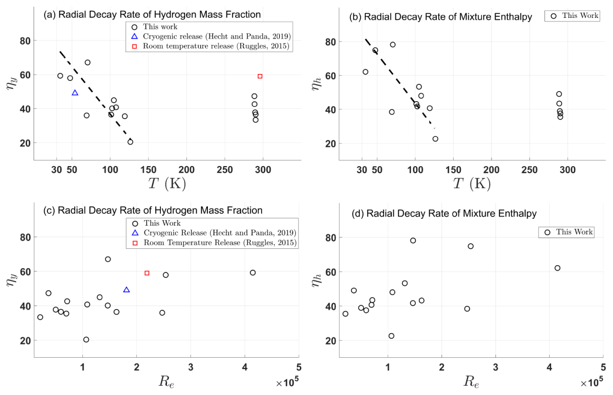
Figure 11
Radial decay rate of mass fraction and enthalpy as a function of release temperature (a, b) and jet Reynolds number (c, d). Experimental data from this work (black circles), cryogenic literature data (blue triangles) (Hecht and Panda, 2019), room temperature literature data (red squares) (Ruggles, 2015). The dashed line in (a) and (b) indicates the trend of decay rate for the cryogenic jets measured in this work.
3.3 Estimation of turbulent transport parameters
According to Kleinstein’s analysis, the ratio of the axial decay rates of dimensionless velocity and normalized mixture enthalpy can be interpreted as Prt. Similarly, the ratio of dimensionless velocity and mass fraction represents Sct. Since this work did not measure the jet velocity, we estimate the Let along the axial direction using the decay rate ratio of mixture enthalpy and mass fraction, that is, . The result is shown in Figure 12(a) and (c) as a function of the release temperature and jet Reynolds number, respectively. A linear fitting is proposed, excluding the 35 and 48 K cases, which are not in conformity with the hyperbolic relations (equation (1)). In the radial direction, Kleinstein’s treatment showed that the ratio of the Gaussian coefficient for the mass fraction and enthalpy, that is, , represents the Let. Figure 12(b) and (d) plots the Let along the radial direction where the Gaussian coefficient ratio was obtained by averaging the ratios at different locations (Table 4).
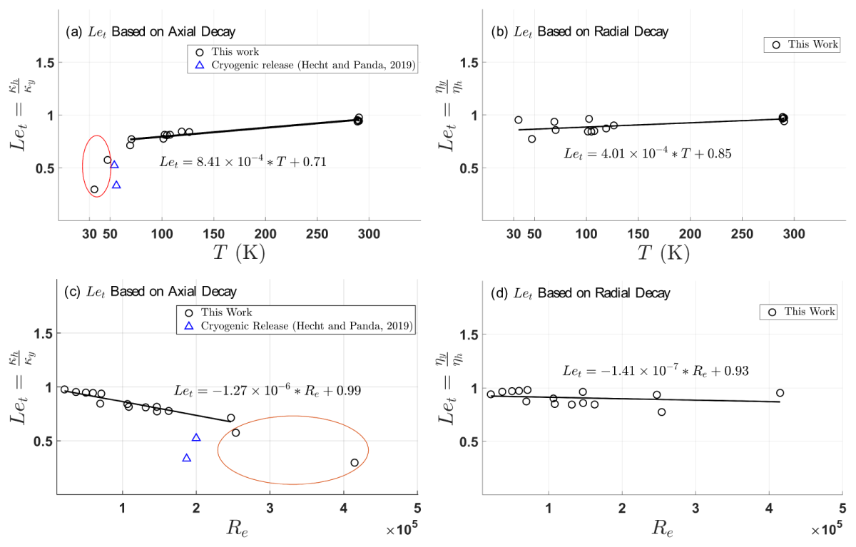
Figure 12
Let as a function of the release temperature, based on (a) the ratio of axial decay rates for enthalpy and mass fraction, and (b) the ratio of radial decay rates for mass fraction and enthalpy. The Let fitting for release temperature at 70 K or higher (35 and 50 K neglected and circled in red). Same Let plotted as a function of jet Reynolds number in (c) and (d). Experiment data from this work (black circle), literature data (blue triangle) (Hecht and Panda, 2019).
Despite the considerable scattering in Figures 9 and 11 among individual decay rates, the calculated Let collapse into a rather tight band. Let is shown to increase with release temperature and decrease with Reynolds number. The dependence of Let on release temperature and Reynolds number appears to be stronger in the axial direction than in the radial direction, even discarding the 35 K and 48 K cases. On the other hand, at room temperature, Let in both directions reaches approximately 0.95, close to the typically assumed value of 1 in CFD simulations (Giannissi and Venetsanos, 2018; Saini et al., 2024). Similar to our 35 and 50 K cases, the Let derived from the Sandia experiments are also well below 1, which is worth exploring in future work. A smaller Let, for example, 0.85, has been used in previous simulations of cryogenic hydrogen release (Giannissi et al., 2021).
The experimentally determined Let can be used to estimate Prt and Sct using the velocity decay rate from the CFD simulation. An example result for the 103 K/506 KPa release case is shown in Table 5, using the CFD method reported in Saini et al. (2024). The Prt is calculated to be 0.96 along the axial direction and 0.67 along the radial direction. This indicates that the transport of enthalpy and momentum is at a similar rate in the axial direction, but that enthalpy is transported faster than momentum in the radial direction, which can be explained by the stronger axial momentum. The Prandtl numbers (Pr) based on molecular properties are approximately 0.75 for air and 0.68 for hydrogen between 100 and 300 K, which is similar to Prt in the radial direction. This suggests that the radial decay is largely controlled by molecular diffusion, which is supported by Figure 11 where the jet Reynolds number shows little impact on the radial decay rates.
Table 5
Turbulent Prt and Sct estimation for release at 103 K, 506 KPa.
| PARAMETERS | VALUE | |
|---|---|---|
| Axial decay rate | Mass fraction κy | 0.199 (measured) |
| Enthalpy κh | 0.162 (measured) | |
| Velocity κv | 0.156 (CFD) | |
| Axial turbulent parameters | 0.81 (measured) | |
| 0.96 (calculated using CFD) | ||
| 0.78 (calculated using CFD) | ||
| Radial decay rate | Mass fraction ηy | 40.5 (measured) |
| Enthalpy ηh | 41.5 (measured) | |
| Velocity ηv | 62 (CFD) | |
| Radial turbulent parameters | 0.96 (measured) | |
| 0.67 (calculated using CFD) | ||
| 0.65 (calculated using CFD) | ||
3.4 Two-dimensional hydrogen concentration contour
To evaluate the impact of release temperature on the size of flammable envelope, two-dimensional contours of hydrogen concentrations are constructed using the centreline measurements and the average Gaussian function fitted from the radial measurements at the same condition. Figure 13 shows the results for release temperature at 35–290 K at a fixed release pressure of 300 kPa, indicating a larger hydrogen concentration contour as the release temperature decreases (where mass flow rate increases).
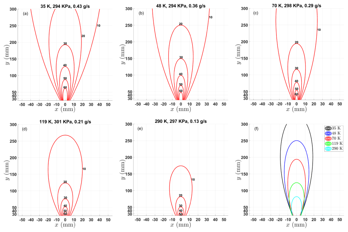
Figure 13
Hydrogen mole fraction (%) contour at different release temperatures and a fixed release pressure of 300 KPa: (a) 35 K, (b) 48 K, (c) 70 K, (d) 119 K, (e) 290 K and (f) contours of 20% H2 mole fraction at different release temperatures.
Figure 14 shows the hydrogen concentration contour for release temperature at 35–289 K at a fixed mass flow rate of 0.43g/s, which also shows a larger hydrogen concentration contour at lower release temperature. The longer contour can be explained by the slower axial decay of colder jets, as shown in Figure 9. The wider contour apparently contradicts the faster radial decay of colder jets in Figure 11. However, the radial decay is relative to its centreline concentration, which decays more slowly with colder jets. The combination of the two effects results in a longer and wider contour for cold jets, indicating a deeper jet penetration as well as a higher volume of flammable gas, both suggesting a larger separation distance compared to the room temperature release at comparable release pressure or mass flow rate.
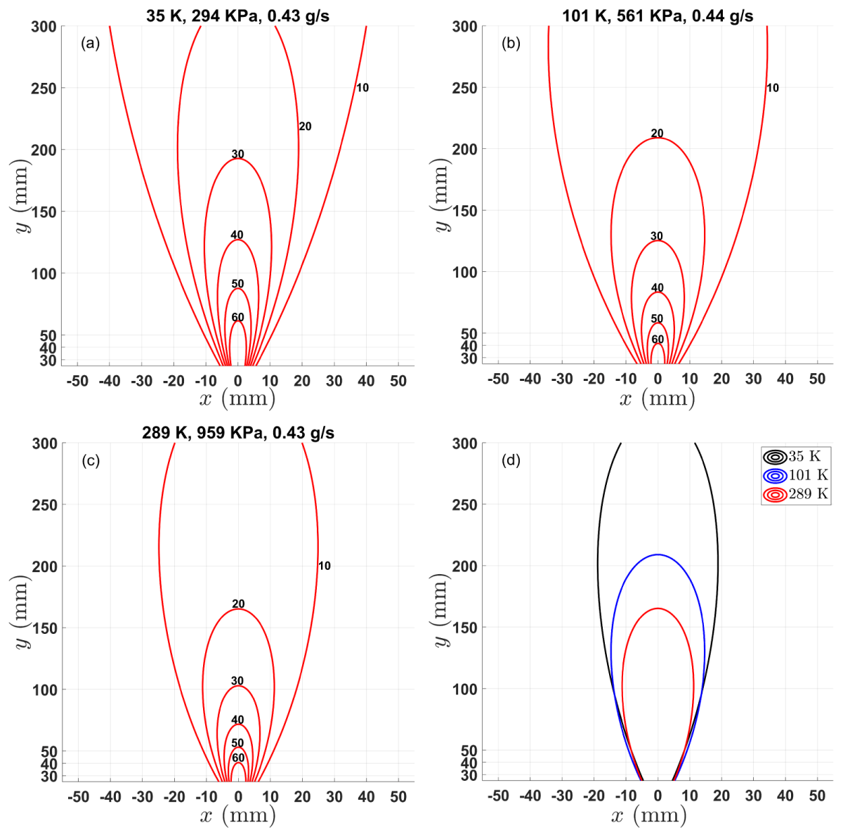
Figure 14
Hydrogen concentration contour at different release temperatures and a fixed mass flow rate of 0.43 g/s: (a) 35 K, (b) 101 K, (c) 289 K and (d) contours of 20% H2 mole fraction at different release temperatures.
3.5 Adiabatic mixing
The adiabatic mixing assumption is examined using the cryogenic release data (35–126 K) in this work. The mixing equation is written as
where XH2 is hydrogen molar fraction and T_mix is the mixture temperature. is the molar-based specific heat and the subscript e, ∞ and mix indicating the value at the temperature of the nozzle exit, ambient and mixture, respectively.
Figure 15 shows both the experimentally measured hydrogen mole fraction (XH2,measured) and the calculated hydrogen mole fraction (XH2,calculated) using the adiabatic mixing equation (equation (7)). All data points generally collapse onto a straight line with a slope of 1.06, with some outliers at both ends of the measured range. At high H2%, the deviation could be due to air condensation; at low H2%, it could be due to the error in measuring small hydrogen concentrations (±2 vol%). Although this result proves adiabatic mixing is generally applicable to cryogenic jet mixing, an accurate correlation between species concentration and mixture temperature must take into account the deviation from the 1:1 fitting.
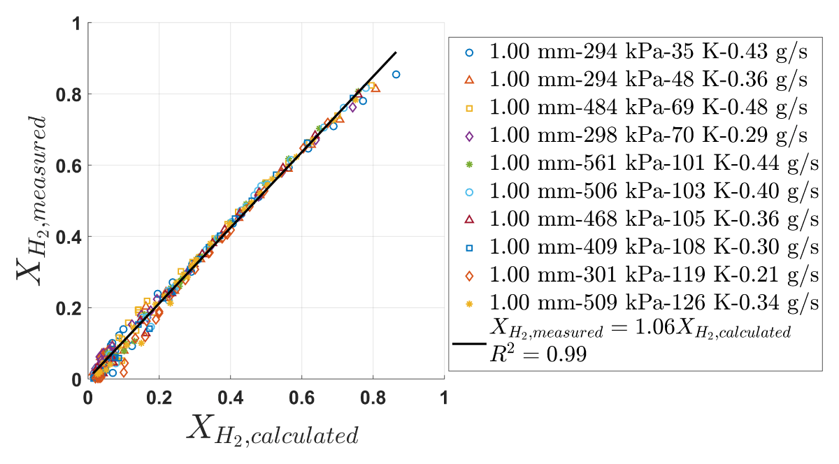
Figure 15
Examination of the applicability of adiabatic mixing to the cryogenic release experiments. XH2,calculated is from equation (7). Both axial and radial measurements are plotted; the black line is the linear fitting of all plotted data. A slope of 1 means perfect adiabatic mixing.
3.5 Comparison with HyRAM simulation
Simulation using HyRAM+ 6.0 (Ehrhart et al., 2025) is conducted for all the cases investigated. The results for the release temperature sweep at 300 kPa are presented below. The remaining results are reported in the Supplementary Materials. To account for the presence of the sampling probe in the jet, simulation results are averaged over a circular cross-section of 1.5 mm diameter (corresponding to the probe inner diameter) for comparison with measurements. A revised HyRAM code has been published (Saini et al., 2025) of which the simulation results are also included in the Supplementary Materials.
3.5.1 Axial molar fraction and temperature
Figure 16 compares the simulated hydrogen molar fraction and mixture temperature along the axial direction. HyRAM appears to underpredict both parameters at the same time, which is in contradiction with the adiabatic mixing discussed above; for example, a higher hydrogen concentration should lead to a lower gas temperature. The underprediction of mole fraction is more severe near the nozzle (less than 40 mm above the nozzle) at release temperatures below 70 K. One potential contributor might be the condensation of air components in this region, which could increase local gas temperature and hydrogen mole fraction simultaneously. Nevertheless, the overall HyRAM prediction for centreline concentration and temperature is satisfactory.
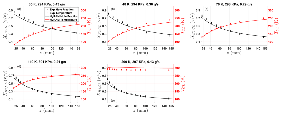
Figure 16
Comparison of measured and simulated centreline hydrogen molar fraction and mixture temperature at different release temperatures and a fixed release pressure of 300 kPa: (a) 35 K, (b) 48 K, (c) 70 K, (d) 119 K and (e) 290 K; symbols for experiment data and curves for HyRAM simulation; black for hydrogen mole fraction and red for mixture temperature.
3.5.2 Radial molar fraction and temperature
Figure 17 compares the measured and simulated radial decay for normalized hydrogen mole fraction and mixture temperature. The simulation reproduces the measured mole fraction and temperature well for the deep cryogenic release (35–70 K). The mixture temperature is almost constant for the room temperature release and therefore cannot be fitted by Gaussian functions. As the release temperature increases, larger discrepancies are observed for the 119 K and room temperature cases. These results indicate that HyRAM needs to improve the radial simulation for release temperatures above 100 K. Similar results are observed in other datasets reported in the Supplementary Materials.
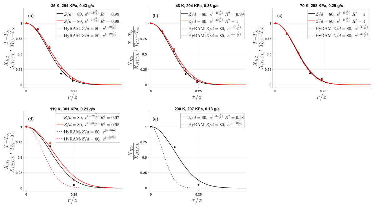
Figure 17
Comparison of the measured and simulated radial hydrogen mole fraction and mixture temperature at different release temperatures and a fixed release pressure of 300 kPa, (a) 35 K, (b) 48 K, (c) 70 K, (d) 119 K and (e) 290 K; solid lines are fitted from measurements (markers) and dashed lines represent results from the HyRAM+ 6.0 simulation; black for hydrogen mole fraction and red for mixture temperature.
The problem of simulating room temperature release has been reported with previous versions of HyRAM (Ehrhart et al., 2021). Part of this can be attributed to some empirical constants being (over)tuned for deep cryogenic conditions. For example, the spreading ratio (λ) for the relative decay of velocity and mass fraction/temperature fields was reduced from 1.5 (version 2.0) to 1.16 (version 3.1 and later versions), which improved the simulation of cryogenic releases but worsened the simulation of room temperature cases (Ehrhart et al., 2021). It is also noted that there is no differentiation of concentration and temperature decay in the HyRAM simulation.
4. Conclusions
This work investigates turbulent axisymmetric hydrogen jet mixing with ambient air in a controlled environment under systematically varied release conditions of 35–290 K, 300–950 KPa and 0.13–0.43 g/s. The hydrogen concentration and gas temperature were measured across the mixing jet using a movable sampling probe with two degrees of freedom. The decays along the axial and radial directions were analysed using Kleinstein’s method. The major conclusions are as follows:
Under cryogenic release conditions, the axial decay rate of the hydrogen mass fraction and the mixture enthalpy, as described by κy and κh in the hyperbolic function (equation (1)), both decreased with decreasing release temperature, indicating slower axial mixing with a colder jet.
In the radial direction, the decay rate of the hydrogen mass fraction and the mixture enthalpy, as described by ηy and ηh in the Gaussian distribution function (equation (3)), both increased with decreasing release temperature, indicating faster radial mixing with a colder jet.
Combining the axial and radial effects, cryogenic hydrogen jets produced a longer and larger flammable envelope.
The turbulent Lewis number was estimated using κh/κy along the axial direction, and ηy/ηh along the radial direction, which greatly reduced the scattering among the individual decay rates. With decreasing release temperature, Let decreased in both axial and radial directions, whereas the axial Let depended more on release temperature. The room temperature value of Let returned to 0.95 in both directions.
The HyRAM simulation reproduced the axial and radial measurements reasonably in most cases, but the performance deteriorated with increasing release temperature. This is likely due to the identical, temperature-invariant decay rates assumed for hydrogen concentration and mixture temperature in the simulation.
These results demonstrated the slower decay with cryogenic jets and call for additional prudence in evaluating the consequence of liquid hydrogen leaks. Future work is therefore recommended on the velocity decay in cryogenic jets and the extension of Kleinstein’s analysis to deep cryogenic conditions. This will help to provide key inputs (turbulent transport properties) to CFD simulations and low-order models.
Additional File
The additional file for this article can be found as follows:
Supplementary Materials
The measured hydrogen concentration and mixture temperature data are provided in the Supplementary Materials. Available at: https://doi.org/10.58895/hysafe.79.s1
Notes
[1] Attempts have been made to determine the enthalpy decay for the Sandia experiments (Hecht and Panda, 2019); however, fitting the radial distribution with the Gaussian function yielded R2 < 0.7, likely due to the cryogenic conditions and measurement uncertainty. Thus, no literature data was included in Figure 11(b) and (d).
Author Contributions
Qiang Ge: Investigation, formal analysis, writing—original manuscript. Zhenbiao Zhou: Investigation, methodology, formal analysis, supervision, writing—review and editing. Daniel Creedon: Methodology, writing—review and editing. Yi Yang: Conceptualization, formal analysis, methodology, funding acquisition, project administration, supervision, writing—review and editing. Michael Brear: Conceptualization, methodology, funding acquisition, writing—review and editing. Deepak Saini: Formal analysis, writing—review and editing. Joe Berry: Formal analysis, funding acquisition, writing—review and editing. Mohsen Talei: Formal analysis, funding acquisition, writing—review and editing. Richard Sandberg: Formal analysis, funding acquisition, writing—review and editing. Melissa Kozul: Formal analysis, funding acquisition, writing—review and editing.