
Table 1
Input uncertainty distributions.
| NAME | DISTRIBUTION | DESCRIPTION |
|---|---|---|
| valve-i | i = 0.01; Log–normal (–5.9, 0.2) i = 0.1; Log–normal (–7.4, 0.4) i = 1.0; Log–normal (–9.8, 1.1) i = 10; Log–normal (–10.6, 0.6) i = 100; Log–normal (–12.2, 1.4) | Default probability distribution for valves for each leak size i ∈ {0.01,0.1,1,10,100} |
| instrument-i | i = 0.01; Log–normal (–7.4, 0.7) i = 0.1; Log–normal (–8.5, 0.8) i = 1.0; Log–normal (–9.1, 0.9) i = 10; Log–normal (–9.2, 1.1) i = 100; Log–normal (–10.2, 1.5) | Default probability distribution for instruments for each leak size i ∈ {0.01,0.1,1,10,100} |
| joint-i | i = 0.01; Log–normal (–10.3, 0.2) i = 0.1; Log–normal (–12.3, 0.9) i = 1.0; Log–normal (–11.8, 0.5) i = 10; Log–normal (–11.8, 0.6) i = 100; Log–normal (–12, 0.7) | Default probability distribution for joints for each leak size i ∈ {0.01,0.1,1,10,100} |
| hose-i | i = 0.01; Log–normal (–7.5, 0.4) i = 0.1; Log–normal (–8.5, 0.6) i = 1.0; Log–normal (–8.7, 0.6) i = 10; Log–normal (–8.8, 0.6) i = 100; Log–normal (–9.7, 1.0) | Default probability distribution for hoses for each leak size i ∈ {0.01,0.1,1,10,100} |
| pipe-i | i = 0.01; Log–normal (–11.7, 0.7) i = 0.1; Log–normal (–12.5, 0.7) i = 1.0; Log–normal (–13.9, 1.3) i = 10; Log–normal (–14.6, 1.2) i = 100; Log–normal (–15.7, 1.8) | Default probability distribution for pipes for each leak size i ∈ {0.01,0.1,1,10,100}. Every 1 meter of pipe is considered a separate pipe component. |
| noz_po_dist | Beta (0.5, 610415.5) | Default probability distribution for nozzle pop-off (disconnection) |
| overp_dist | Beta (3.5, 310289.5) | Default probability distribution for an overpressure during fueling |
| pvalve_fto_dist | Log–normal (–11.74, 0.67) | Default probability distribution for pressure relief valve failure to open |
| driveoff_dist | Beta (31.5, 610384.5) | Default probability distribution for accidents due to drive-off during refueling |
| coupling_ftc_dist | Beta (0.5, 5031) | Default probability distribution for breakaway coupling failure to close |
| x_i_location | Uniform (1, 20) [m] | Independently sampled for each occupant i ∈ {1,2,…N} |
| z_i_location | Uniform (1, 12) [m] | Independently sampled for each occupant I ∈ {1,2,…N} |
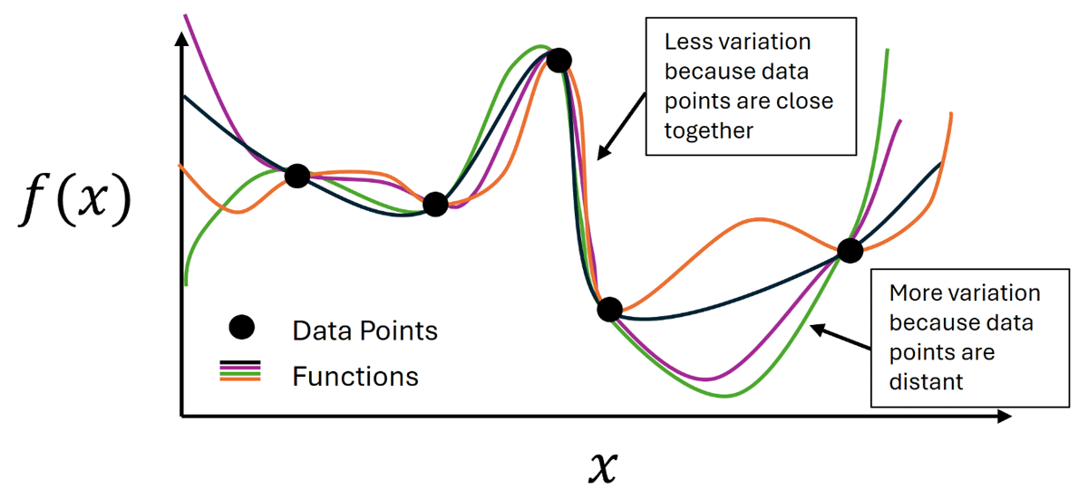
Figure 1
Illustration of the Gaussian Process model concept: for data points near each other in the input space, there is less uncertainty, which results in less variation between functions. For interpolations between distant points, there is more variation.
Table 2
Descriptions of the different cases included in the sensitivity analysis.
| SAMPLE STRUCTURE | CASE 1: BASE CASE | CASE 2: OCCUPANTS MOVED CLOSER TO LEAKS | CASE 3: DOUBLING OF SYSTEM PRESSURE | CASE 4: OCCUPANTS MOVED CLOSER TO LEAK AND DOUBLING OF SYSTEM PRESSURE | ||||
|---|---|---|---|---|---|---|---|---|
| SINGLE LOOP | DUAL LOOP | SINGLE LOOP | DUAL LOOP | SINGLE LOOP | DUAL LOOP | SINGLE LOOP | DUAL LOOP | |
| Number of Occupants | 1 | 9 | 1 | 9 | 1 | 9 | 1 | 9 |
| Number of Samples | 2000 | N = 125 M = 40 | 2000 | N = 125 M = 40 | 2000 | N = 125 M = 40 | 2000 | N = 125 M = 40 |
| X Loc. ~ uniform [m] | 1–20 | 0.01–1 | 1–20 | 0.01–1 | ||||
| Z-Loc. ~ uniform [m] | 1–12 | 0.01–0.02 | 1–12 | 0.01–0.02 | ||||
| Pressure [MPa] | 35 | 35 | 70 | 70 | ||||
[i] Note: N is the sample size for the location sampling loop; M is the sample size for the non-location parameter loop.
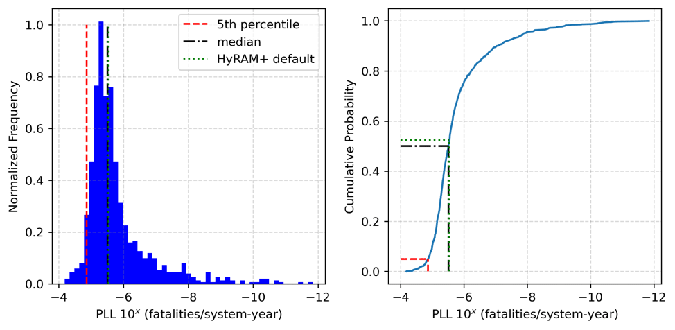
Figure 2
Uncertainty quantification results generated by propagating 1,000 LHS samples through HyRAM+ QRA calculations. The left plot shows a histogram of the PLL, while the right plot shows the empirical cumulative distribution frequency. Median, 5th percentile, and deterministic HyRAM+ results are highlighted on both plots.
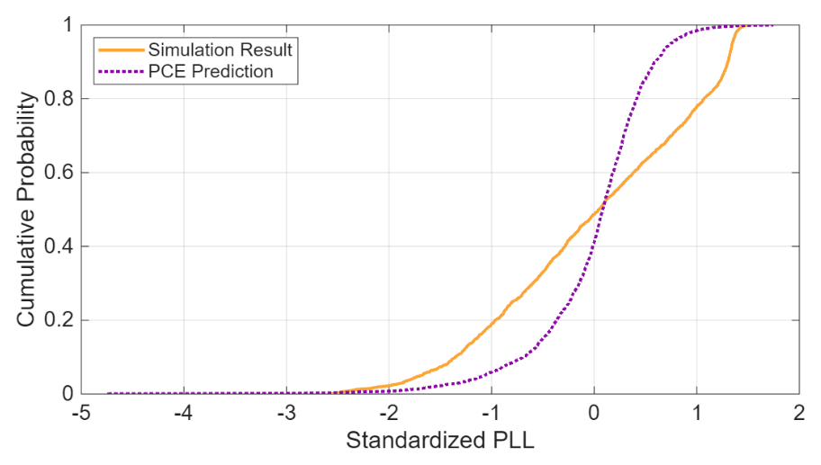
Figure 3
Comparison between the empirical CDFs of the simulation results and the regression predictions for the Case 1 single loop analysis.
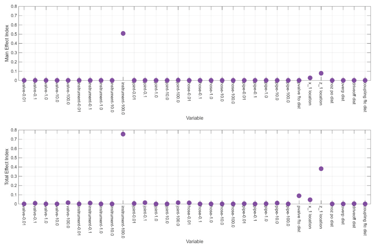
Figure 4
Main (top) and total (bottom) effect indices for the Case 1 single-loop analysis identify the instrument rupture frequency and location of the occupant relative to the leak as the most important factors affecting PLL.
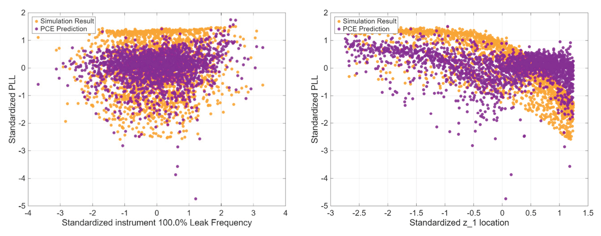
Figure 5
Comparison of the simulation results and regression results from the Case 1 single-loop analysis for the instrument rupture frequency (left) and z-location (right) versus the standardized PLL.
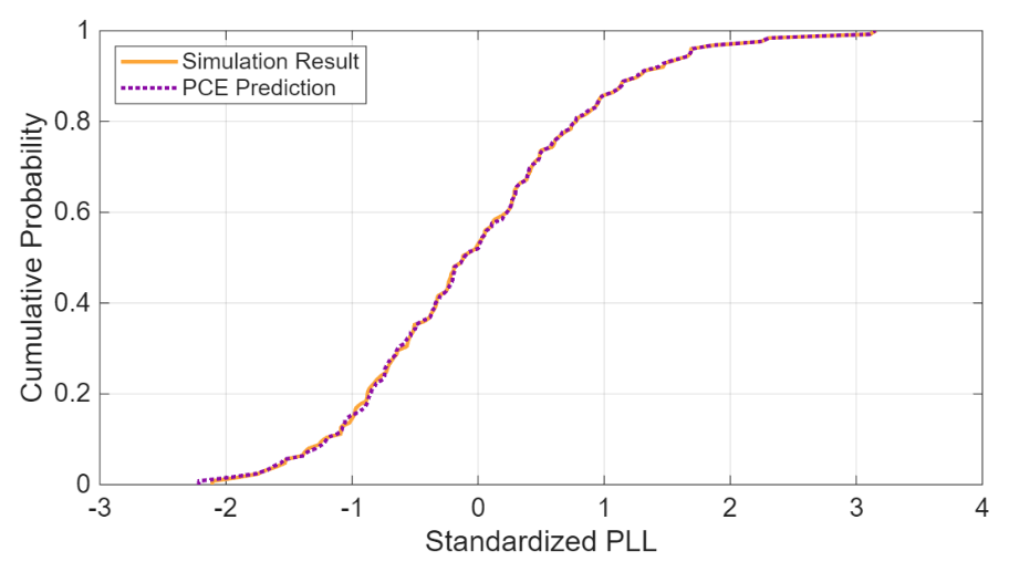
Figure 6
Comparison between the empirical cumulative distribution functions of the simulation results and the surrogate predictions for the Case 1 dual-loop analysis indicates a good fit in the regression analysis for PLL.
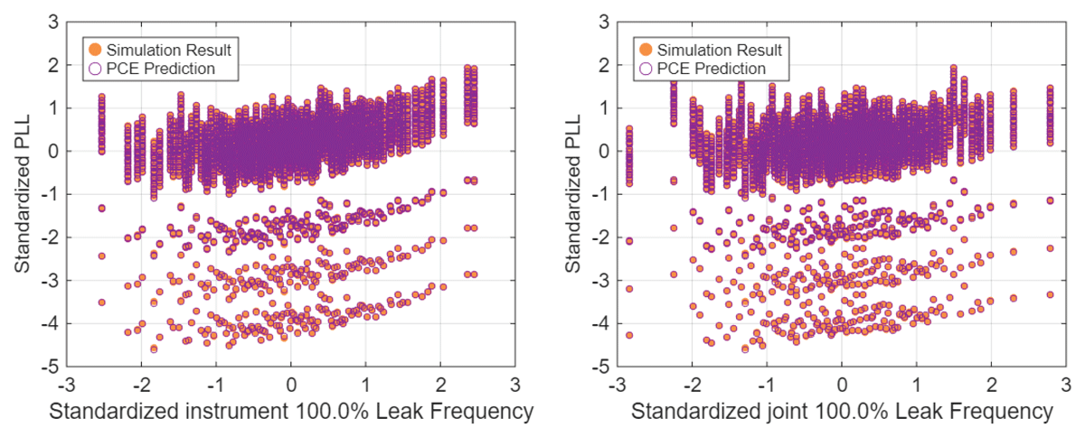
Figure 7
Comparison of the simulation results and regression results from the Case 1 dual-loop analysis for the standardized instrument rupture frequency (left) and standardized joint rupture frequency (right) versus the standardized PLL.
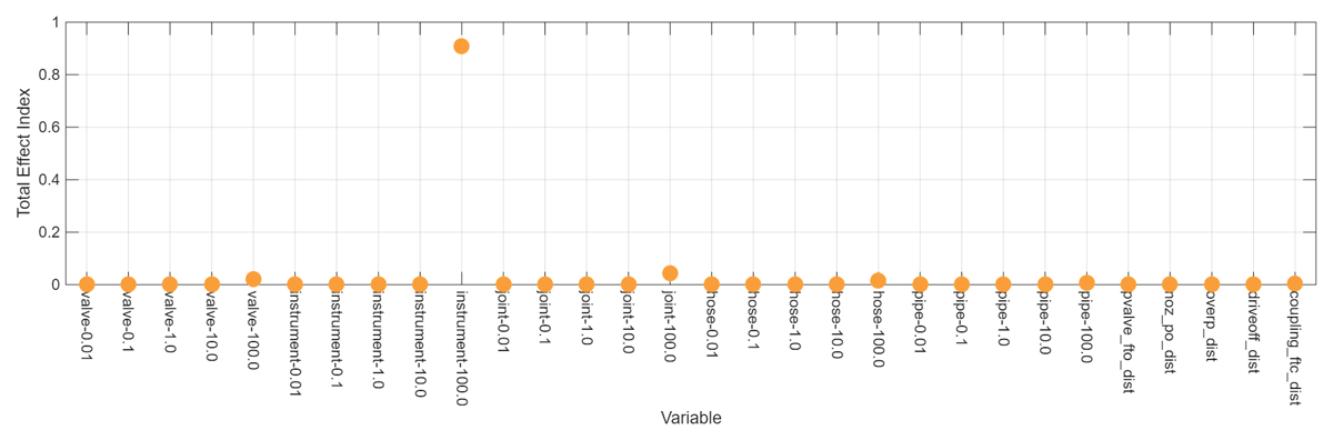
Figure 8
Total effect sensitivity indices for the Case 1 dual-loop analysis.
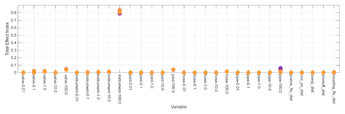
Figure 9
Total effect sensitivity indices for the Case 2 dual-loop analysis with different colors denoting different occupant location realizations.