
1.0 Introduction
It is necessary to understand the safety risks related to continued development and deployment of hydrogen infrastructure. Risk assessments can be used to inform siting approval, prioritize maintenance activities, or inform design or operational changes. The Hydrogen Plus Other Alternative Fuels Risk Assessment Models (HyRAM+) software is a publicly available, open-source toolkit that can be used to support this need. HyRAM+ provides deterministic risk predictions for specific system configurations. However, it is important to quantitatively incorporate uncertainty into these predictions; uncertainty quantification (UQ) and sensitivity analysis (SA) allow risk prediction results to be interpreted and utilized correctly.
This article discusses the development of UQ and SA tools for HyRAM+ using a default indoor hydrogen forklift fueling facility model (Groth et al., 2012). HyRAM+ is used, deterministically, to predict risk for the facility as an example. For this quantitative risk assessment (QRA), the characterization of risk provided by Kaplan and Garrick (Kaplan and Garrick, 1981) is used, wherein risk is a triplet of information that answers the following three questions:
What can go wrong?
How likely is it?
What are the consequences?
Treatment of uncertainty and sensitivity in this work focuses around the second question, as there is high uncertainty about the likelihood of such events. If knowledge about such a system were complete and there were no stochastic variation, a deterministic QRA computation that answers these questions would be sufficient for informing risk decisions. However, the state-of-knowledge may not be complete, especially for developing technologies like hydrogen infrastructure. Incorporating uncertainty into the answers to these questions can provide valuable insights into the level of uncertainty surrounding risk predictions and the driving factors contributing to that uncertainty. In this work, this is accomplished by propagating varied values of input parameters through the deterministic HyRAM+ model. Uncertainty in the input parameters may come from a variety of sources, including limited data, installation/maintenance differences, and human factors. UQ is performed to describe the output uncertainty, and SA is used to identify the most important input uncertainties contributing to the uncertainty in risk. This is not a complete treatment of all uncertainties related to modeling hydrogen safety risk; there are sources of uncertainty that are not included in this analysis, such as model form uncertainty in the probit models used to predict fatalities or the physical models used to predict harm exposures.
2.0 Methodology
2.1 Risk model
The demonstration system for this analysis is an indoor gaseous hydrogen forklift fueling facility (Groth et al., 2012) with the default parameters used in HyRAM+. Gaseous hydrogen for this system is at 287.7 K (~60°F) and 35 MPa (5076 psi absolute). The ambient conditions are assumed to be 288 K (59°F) and 101,325 Pa (14.7 psi) with 89% relative humidity. The system consists of 5 valves, 3 instruments, 35 joints, 1 hose, and 20 meters of pipe. Each meter of pipe is treated as a separate component, and the pipe is the same diameter throughout, with an outer diameter of 0.375 inches (9.525 mm) and a wall thickness of 0.065 inches (1.651 mm). The system includes refueling capability and can consider potential failures for 20 vehicles, 2 fueling operations per vehicle per day, and over 250 days per year (10,000 fueling operations annually). It is assumed that there are nine facility occupants, and they are randomly distributed between 1 and 20 meters away from a leak in the x direction (direction of the leak), and between 1 and 12 meters away from the leak in the z direction (tangential to the leak) and are standing at ground level. An exclusion radius of 0.01 m (<0.5 in) is assumed; occupants cannot enter this region in the model. The probability of a leak being detected and mitigated before it can ignite is assumed to be 0.9 (90%).
The Yüceil/Ötügen notional nozzle model is used for leak modeling (Sandia National Laboratories, 2024). The discharge coefficient is assumed to be 1, and the leak is assumed to be a horizontal leak at ground level. Ignition probabilities for leaks are specified as a function of the leak mass flowrate for both immediate and delayed ignition (Tchouvelev, 2008).
Depending on leak characteristics and the timing of ignition, an ignited leak may produce a steady-state jet flame or an explosion. HyRAM+ calculates three-dimensional heat flux responses for jet flames and peak overpressure for explosions; the peak overpressure calculation uses the Baker–Strehlow–Tang (BST) method with a Mach flame speed of 0.35. Thermal or overpressure probit models (i.e., fatality models) are applied to estimate the consequences to occupants of leak events (Sandia National Laboratories, 2024; Schroeder and Brooks, 2024). For probit models that require conversion from heat flux to thermal dose, an exposure time of 30 seconds is assumed.
HyRAM+ combines an event sequence diagram with fault trees to apply these risk calculations for the total system. Fault trees calculate the overall system frequency of a leak of a specific size occurring by combining the frequencies of leaks of that size over all components. For example, fault trees calculate the overall system leak frequency for a given leak size based on the corresponding leak frequencies for that leak size for all valves, instruments, joints, hoses, and meters of pipe. This frequency is then input to an event sequence diagram that determines the frequency of different outcomes (shutdown, no ignition, jet fire, and explosion) based on the probabilities of intermediate events, such as leak detection and isolation, or immediate/delayed ignition.
The heat flux and overpressure responses are calculated for each leak event modeled with the combined event/fault tree model. The probit models are applied to estimate fatality probabilities for all occupant locations. The overall risk is calculated by adding the fatality probabilities over all consequences (heat flux and overpressure), all locations, and all leak sizes. This measure is called the potential loss of life (PLL) and is the only risk metric considered in this analysis. The UQ and SA methods discussed here would apply without loss of generality to any risk measures calculated by HyRAM+.
2.2 Uncertainty analysis
Uncertainty in HyRAM+ is characterized probabilistically based on the concept of subjective probability, which arises from Bayesian statistics. Probability from the Bayesian perspective describes the beliefs about an uncertain variable. The structure of this type of analysis is fairly standard for forward propagation of uncertainty. First, probability distributions are derived for uncertain inputs to the QRA model of the refueling station. These distributions define an input space for the deterministic QRA model. A large sample of points is drawn from the input space and the QRA model is evaluated at each point. The QRA model outputs a different risk estimate (PLL) at each point in the sample. This distribution of values for the PLL estimate describes the uncertainty around risk.
Two types of uncertainty are considered that can affect QRA results for this forward propagation. The first is epistemic, or state-of-knowledge, uncertainty. This is uncertainty that could potentially be reduced with further study. The other type of uncertainty considered is aleatory uncertainty, or random variation. This is uncertainty that cannot be reduced with further study. Separating uncertainties into these two types is a common practice in uncertainty analysis because it is useful to identify the proportion of uncertainty that is inherent to the problem versus the proportion of uncertainty that could potentially be changed. When uncertainty around a risk is too high for decision-making, this separation can help target efforts for uncertainty reduction.
Some uncertainties in HyRAM+, as in most QRA models, are neither fully epistemic nor fully aleatory. Leak frequencies are an example of this. Leak frequency distributions in HyRAM+ were developed from a broad set of published data from a wide variety of systems (Glover and Brooks, 2023; LaChance et al., 2009). These distributions include the aleatory uncertainty that you would expect to see between different types of systems or different locations of the same basic system design. This uncertainty could be induced by different operating procedures, manufacturers, maintenance procedures, operational time, environmental conditions, etc. Leak frequency distributions also incorporate epistemic uncertainty because the frequency with which a specific valve will leak under the exact same conditions is also not precisely known. In this analysis, the uncertainties are partitioned only for convenience because some of them are a mixture of aleatory and epistemic effects and do not fit cleanly into either category.
Sampling
One type of sampling design was performed on the risk assessment model for UQ, and another type for SA. The UQ study does not separate the two types of uncertainty. All of the uncertain variables are sampled together; each sampled point consists of a new randomly selected value for each uncertain variable. A sample size of 1,000 was used for this UQ.
For SA, the uncertain variables were also separated into a dual-loop sampling structure. The occupant locations were sampled in one loop, and all of the other uncertain variables were sampled in the other loop. This results in a sample with the following structure.
The location sample is {L1,L2,L3,…,LN}, where each point Li consists of sampled locations for all occupants. In other words, each Li is an occupant location configuration and there are N-many different occupant configurations. For the other sampling loop, all of the non-location uncertain parameters were sampled. This sample is {P1,P2,P3,…,PM}, where each point Pj consists of a sampled value for all of the non-location uncertain parameters. The deterministic model was evaluated at each Pj for each occupant configuration Li. In other words, a single realization of the QRA model was evaluated at {Li, Pj}, and all possible combinations of Li and Pj are included. The total sample size is N × M, though this sample includes repeated information because the {P1,P2,P3,…,PM} samples are repeated N-times.
The downside of this sampling structure is that the sample contains less information than it would if a different set of Pj samples was drawn for each occupant location configuration. The benefit of this sampling structure is that subsets of the sample space can be examined to see how much of an impact the location has versus all of the other parameters. For example, if the collection of realizations {L1,P1},{L1,P2},{L1,P3},…,{L1,PM} is considered, the occupant location configuration is constant within this set of realizations, so any variation in PLL across these realizations can be attributed exclusively to the non-location parameters. Similarly, if the collection of input points {L1,P1},{L2,P1},{L3,P1},…,{LN,P1} is considered instead, then all of the variation in PLL across these realizations can be attributed exclusively to the occupant locations. The sample sizes used in these SA studies are shown in Table 2.
Sampling was performed using Latin hypercube sampling (LHS) with the Python LatinHypercube function in SciPy’s Quasi-Monte Carlo submodule of the Statistical Functions module (Virtanen et al., 2020). LHS sampling is a stratified sampling technique that enforces a more uniform coverage of the sample space than simple random sampling (Helton and Davis, 2001). This implementation of LHS stratifies the sample space and then takes a random sample within each stratum (as opposed to the midpoint of the stratum, as is the case in some implementations).
Input uncertainties
This analysis considered a subset of uncertain HyRAM+ parameters: component leak frequencies, dispenser failure probabilities, and occupant locations. The same methods would apply if expanding the uncertainty space to more parameters, but may require larger sample sizes. Uncertainties for these parameters are already included in HyRAM+ (Ehrhart et al., 2023), though only the mean or median values are used in deterministic QRA calculations. Therefore, no new uncertainty distributions were developed for this analysis. It is important to emphasize that these are not the only potential sources of uncertainty in QRA calculations; these sources of uncertainty were chosen for convenience to demonstrate the methodology using existing uncertainty distributions, not as a claim of total uncertainty in a QRA calculation. There are many other inputs in the HyRAM+ QRA calculation that are not sampled here, and there are many other potential sources of uncertainty that are not explicitly considered in the current HyRAM+ QRA calculation. These input uncertainty distributions may reflect a lack of knowledge about the true value, but may also reflect variability in component types, maintenance differences, or human factors interactions.
The uncertain parameters and their distributions are shown in Table 1. Log-normal distributions are parameterized by the mean and standard deviation of the parameter’s natural logarithm. Beta distributions are parameterized by the typical beta shape parameters. Uniform distributions are parameterized by the upper and lower bounds of the interval with non-zero density. Leak sizes are expressed as percentages (0.01, 0.1, 1, 10, and 100) of the system pipe internal cross-sectional area.
Table 1
Input uncertainty distributions.
| NAME | DISTRIBUTION | DESCRIPTION |
|---|---|---|
| valve-i | i = 0.01; Log–normal (–5.9, 0.2) i = 0.1; Log–normal (–7.4, 0.4) i = 1.0; Log–normal (–9.8, 1.1) i = 10; Log–normal (–10.6, 0.6) i = 100; Log–normal (–12.2, 1.4) | Default probability distribution for valves for each leak size i ∈ {0.01,0.1,1,10,100} |
| instrument-i | i = 0.01; Log–normal (–7.4, 0.7) i = 0.1; Log–normal (–8.5, 0.8) i = 1.0; Log–normal (–9.1, 0.9) i = 10; Log–normal (–9.2, 1.1) i = 100; Log–normal (–10.2, 1.5) | Default probability distribution for instruments for each leak size i ∈ {0.01,0.1,1,10,100} |
| joint-i | i = 0.01; Log–normal (–10.3, 0.2) i = 0.1; Log–normal (–12.3, 0.9) i = 1.0; Log–normal (–11.8, 0.5) i = 10; Log–normal (–11.8, 0.6) i = 100; Log–normal (–12, 0.7) | Default probability distribution for joints for each leak size i ∈ {0.01,0.1,1,10,100} |
| hose-i | i = 0.01; Log–normal (–7.5, 0.4) i = 0.1; Log–normal (–8.5, 0.6) i = 1.0; Log–normal (–8.7, 0.6) i = 10; Log–normal (–8.8, 0.6) i = 100; Log–normal (–9.7, 1.0) | Default probability distribution for hoses for each leak size i ∈ {0.01,0.1,1,10,100} |
| pipe-i | i = 0.01; Log–normal (–11.7, 0.7) i = 0.1; Log–normal (–12.5, 0.7) i = 1.0; Log–normal (–13.9, 1.3) i = 10; Log–normal (–14.6, 1.2) i = 100; Log–normal (–15.7, 1.8) | Default probability distribution for pipes for each leak size i ∈ {0.01,0.1,1,10,100}. Every 1 meter of pipe is considered a separate pipe component. |
| noz_po_dist | Beta (0.5, 610415.5) | Default probability distribution for nozzle pop-off (disconnection) |
| overp_dist | Beta (3.5, 310289.5) | Default probability distribution for an overpressure during fueling |
| pvalve_fto_dist | Log–normal (–11.74, 0.67) | Default probability distribution for pressure relief valve failure to open |
| driveoff_dist | Beta (31.5, 610384.5) | Default probability distribution for accidents due to drive-off during refueling |
| coupling_ftc_dist | Beta (0.5, 5031) | Default probability distribution for breakaway coupling failure to close |
| x_i_location | Uniform (1, 20) [m] | Independently sampled for each occupant i ∈ {1,2,…N} |
| z_i_location | Uniform (1, 12) [m] | Independently sampled for each occupant I ∈ {1,2,…N} |
2.3 Sensitivity analysis
SA identifies the uncertain input parameters that contribute the most to uncertainty in the QRA model output, in this case PLL. It is often performed with UQ because the inputs and outputs of a UQ analysis can be used directly for some SA methods, and the SA further explains the UQ results. In this case, separate sets of simulations were used for UQ and SA because additional cases were added to the SA to investigate specific results. A variance-based SA was chosen, which decomposes the total variance in PLL and apportions it to the variance in the uncertain input parameters. This apportionment is described by main and total effect indices. The main effect index (a dimensionless value) describes what proportion of the variance in the output can be explained by each uncertain input parameter individually, not including any interactions between uncertain input parameters. It can be defined generally, as follows. For uncertain input parameters X1,X2,…,Xd and model output Y(X1,X2,…,Xd), the main effect index for Xk for any k ∈ {1,2,…,d} is
where VarXd is the variance with respect to Xd and EX~d is the expectation with respect to Xk for all k ≠ d (Sobol’, 2001; Sobol’, 1993; Saltelli et al., 2008). Because the denominator for Sk is the same for all uncertain input parameters, . Total effect indices are an extension of main effect indices, which also account for the variance in the output that can be described by interactions between the Xd. The total effect index for Xk is (Sobol’, 2001; Sobol’, 1993; Saltelli et al., 2008)
where VarX~k is the variance with respect to X when all parameters except k are held fixed and EXk is the expectation with respect to Xk. When there are no interaction effects, the main and total effect indices will be equal. When there are interaction effects, the total effect index will always be greater than the main effect index. Unlike the main effect indices, which sum to 100% (or less) than the total variance, the sum of the total effect indices can exceed 1. This is because the interaction effect between two uncertain input parameters is double-counted in the total effect index sum; it is included in the total effect indices for both parameters.
It is useful to first consider the main effect indices; the higher the index, the more sensitive the PLL is to that parameter. For low main effect indices, the PLL is not sensitive. There is no consensus on this threshold; main effect indices below 0.2 or 0.1 are sometimes treated as spurious (Swiler et al., 2021). After looking at the main effect indices, the total effect indices should be considered to see if (1) the total effects are higher, and (2) the total effect indices rank the parameters differently than the main effect indices. In this case, interaction effects may merit additional investigation or explanation. If the total effects indices are essentially the same as the main effects indices, then either set of indices can be used to describe the SA conclusions.
It is not always straightforward to calculate these indices, especially for computationally expensive models, because of the high-dimensional integrals in their calculation. The strategy employed in this work was to approximate the risk model with a fast-running surrogate model, which then estimated Sk and Tk.
This method for SA fits a surrogate model using the sampled input parameters as the independent variables and the resulting PLL samples as the dependent variable. Different surrogate model forms can be used, and typical sampling strategies or estimation techniques can be applied to the surrogate models to estimate Sk and Tk.
Two different surrogate model forms were investigated: polynomial chaos expansion (PCE) and Gaussian Process (GP), both as implemented in Dakota (Adams et al., 2022). The PCE surrogate model is especially useful for SA because it simplifies the estimation of Sk and Tk. A PCE model represents the output as sum of polynomials where the coefficients of the polynomials are random variables. The polynomials are chosen to be orthogonal, and the resulting PCE allows for Sk and Tk to be calculated analytically from the expansion coefficients (Adams et al., 2022). This essentially reduces the problem of sensitivity index estimation to fitting a PCE that approximates the risk model well. PCE models are also generally flexible surrogate models. They allow for discrete and continuous input variables and can describe nonlinear and nonmonotonic input/output relationships well in many cases. However, one particularly useful benefit of PCEs for this model compared to more traditional polynomial (linear, quadratic, etc.) regression models is that PCEs can model non-constant output variance over the input space.
The GP surrogate model does not allow for analytical calculation of sensitivity indices. Instead, the GP surrogate model must be evaluated at many samples in the input space to estimate the expectations and variances in the main and total effect equations. The application of sampling to estimate sensitivity indices can potentially introduce sampling uncertainty. However, because the surrogate model is efficient to evaluate, this uncertainty can be mitigated by using a large sample size. For this analysis, LHS was used with a sample size of 20,000. A GP model is defined as a stochastic process for which any finite set of variables in the process has a joint multivariate Gaussian distribution. It can be conceptualized as a distribution over functions, each of which approximates the input/output relationship in the HyRAM+ simulation data (Swiler et al., 2020). This concept is illustrated in Figure 1. Example data points are shown in a one-dimensional input space. Each curve in the figure is an example function; a GP theoretically includes infinitely many such functions. The uncertainty varies throughout the space depending on where the data points are. GPs can be incredibly powerful for fitting to non-monotonic and non-linear relationships in data.
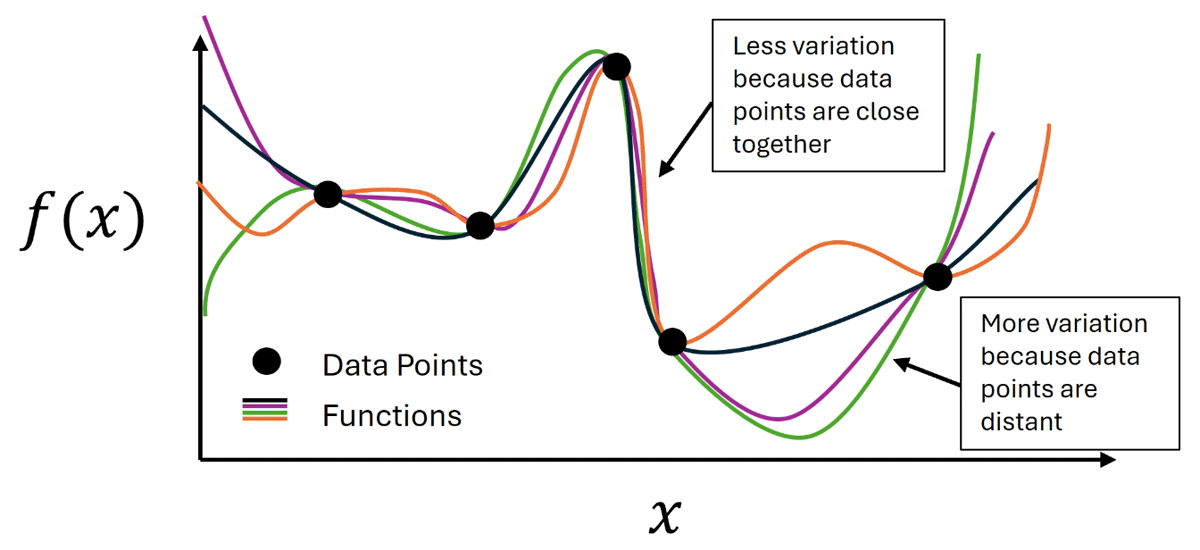
Figure 1
Illustration of the Gaussian Process model concept: for data points near each other in the input space, there is less uncertainty, which results in less variation between functions. For interpolations between distant points, there is more variation.
In single-loop SAs, the surrogate model is fitted to every point that is sampled in the input space. This results in a single sensitivity index estimate for each input risk model parameter. In the dual-loop SA, an independent surrogate model is fitted to every location realization. This results in multiple sensitivity index estimates for each input risk model parameter since there is a different estimate for each location sample.
The Dakota software was used to fit PCEs and GPs for each case and to calculate the sensitivity indices from these models (Adams et al., 2022). GPs generally performed as well or better than PCEs for all cases. When the performance of the GP and PCE was comparable, the PCE was used to estimate sensitivity indices because of the analytical solution for sensitivity indices with PCEs. Performance of the surrogate models was judged qualitatively by visual comparison between the empirical cumulative distribution function (CDF) calculated on the simulation results vs. the empirical CDF calculated on the surrogate model predictions. The input/output scatterplots were also compared between the simulation inputs and outputs and the surrogate model inputs and outputs; this comparison is useful for checking whether the surrogate model accurately describes relationships between the model input and output, whereas the distribution function comparison checks whether the surrogate model accurately describes the output distribution.
The first SA performed was on the set of realizations from the single-loop UQ study. As will be discussed in Section 3.0, this showed that the occupant location overwhelmingly dominates uncertainty. This result motivated the dual-loop UQ study and additional SA studies to interrogate other important uncertainties. This resulted in four sensitivity cases that were studied, described in Table 2. The second case was defined to investigate why non-rupture leaks did not appear to have a significant effect on PLL in Case 1. Occupants were moved closer to the leaks for Case 2 to see if the dominance of rupture (defined as a 100% leak size or complete pipe rupture) on the results was because the occupants were too far from the smaller leaks to receive significant harm. Case 3 was added to see if the system pressure significantly affected which leak sizes dominate risk. Case 4 was added to see if both changes (occupants being closer to leaks and the system pressure being higher) altered the dominance of ruptures in risk. These cases are not an exhaustive list of all possible SA permutations, but rather examples to demonstrate how the SA methodology can be used to interrogate UQ results.
Table 2
Descriptions of the different cases included in the sensitivity analysis.
| SAMPLE STRUCTURE | CASE 1: BASE CASE | CASE 2: OCCUPANTS MOVED CLOSER TO LEAKS | CASE 3: DOUBLING OF SYSTEM PRESSURE | CASE 4: OCCUPANTS MOVED CLOSER TO LEAK AND DOUBLING OF SYSTEM PRESSURE | ||||
|---|---|---|---|---|---|---|---|---|
| SINGLE LOOP | DUAL LOOP | SINGLE LOOP | DUAL LOOP | SINGLE LOOP | DUAL LOOP | SINGLE LOOP | DUAL LOOP | |
| Number of Occupants | 1 | 9 | 1 | 9 | 1 | 9 | 1 | 9 |
| Number of Samples | 2000 | N = 125 M = 40 | 2000 | N = 125 M = 40 | 2000 | N = 125 M = 40 | 2000 | N = 125 M = 40 |
| X Loc. ~ uniform [m] | 1–20 | 0.01–1 | 1–20 | 0.01–1 | ||||
| Z-Loc. ~ uniform [m] | 1–12 | 0.01–0.02 | 1–12 | 0.01–0.02 | ||||
| Pressure [MPa] | 35 | 35 | 70 | 70 | ||||
[i] Note: N is the sample size for the location sampling loop; M is the sample size for the non-location parameter loop.
3.0 Results
3.1 Deterministic and UQ results
The deterministic QRA estimate of risk for the demonstration scenario is 10–5.54 fatalities per system-year. The UQ result with 1,000 samples of the uncertain input space is shown in Figure 2, with statistics and the deterministic result for comparison. The median PLL estimate from the UQ analysis (10–5.51) is close to the deterministic result. This is expected because the nominal values for the deterministic calculation are typically the centers of the uncertainty distributions used in the UQ analysis. There is also significant uncertainty around the median PLL estimate; around 85% of the samples are contained in the interval between 10–8 and 10–5 fatalities per system-year. Based on an understanding of the uncertainty associated with the risk predicted for a system, decision makers can decide to use a more conservative estimate such as the 5th percentile (10–4.82 in this example) or a less conservative estimate such as the median, depending on their application. By understanding the uncertainty in a risk metric calculation, a change to the calculation due to a design change can be put in context to show whether such a risk reduction would be significant or not.
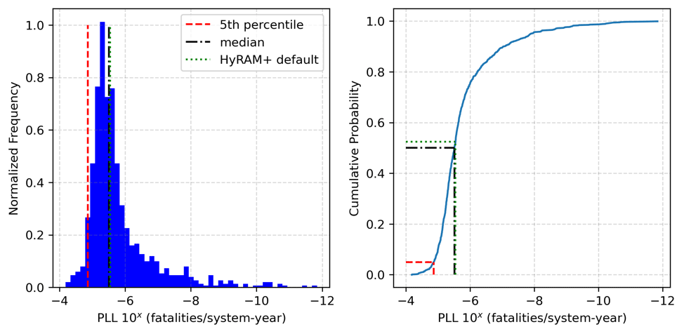
Figure 2
Uncertainty quantification results generated by propagating 1,000 LHS samples through HyRAM+ QRA calculations. The left plot shows a histogram of the PLL, while the right plot shows the empirical cumulative distribution frequency. Median, 5th percentile, and deterministic HyRAM+ results are highlighted on both plots.
3.2 Sensitivity analysis results
Case 1 results
The single-loop sensitivity Case 1 results are shown in Figures 3 and 4. Standardized values are calculated by subtracting the mean from each data point and dividing that difference by the standard deviation. This standardizes the data to have a mean of 0 and a standard deviation of 1, while maintaining the shape of the original data distribution. Figure 3 shows a comparison between the empirical CDFs of the QRA results (solid orange) and the PCE model (purple dashed). This shows that there is significant disagreement between the QRA results and the surrogate model. Figure 4 shows the main and total effect indices from this model. The main effects (top) identify the instrument rupture frequency as the dominant parameter with some potential influence from the occupant location. The total effects (bottom) show significantly more importance from both parameters, with a clearly significant effect from occupant location. This result motivated the use of a dual loop sampling structure; the single-loop PCE model is a poor fit and the PCE model was better able to fit the input/output relationship with the instrument rupture frequency when the input/output relationship with the occupant location was conditioned out. Hence, the relative importance of these variables indicated by the surrogate model is not necessarily accurate.
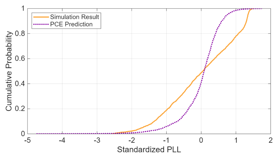
Figure 3
Comparison between the empirical CDFs of the simulation results and the regression predictions for the Case 1 single loop analysis.
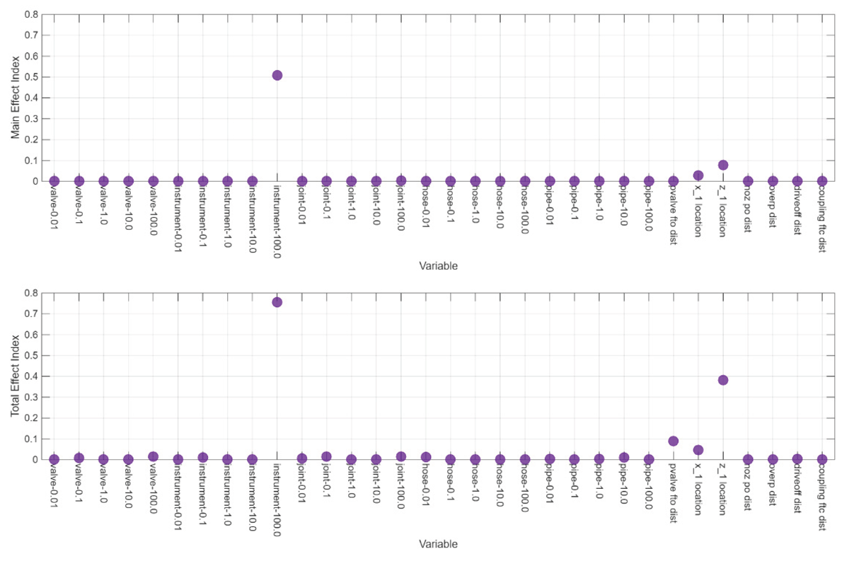
Figure 4
Main (top) and total (bottom) effect indices for the Case 1 single-loop analysis identify the instrument rupture frequency and location of the occupant relative to the leak as the most important factors affecting PLL.
Scatterplots in Figure 5 show the QRA model results (orange) with the predictions from the surrogate model (purple) for the Case 1 single-loop analysis. The subplot on the left compares the relationship between the instrument rupture frequency and the PLL between the QRA model and the surrogate prediction; the subplot on the right does this comparison for the z-location and the PLL. In both cases, the surrogate prediction captures the direction of the trend, but the QRA model results have significant features that are not captured by the surrogate. This is especially the case with the occupant location, where the negative correlation between standardized z-location and standardized PLL is much weaker in the surrogate model; the orange (simulation result) points in this scatterplot show a strong decreasing trend with respect to occupant location. The surrogate failing to capture this trend is likely why the instrument rupture sensitivity indices were higher, even though the scatter plots suggest the z-location sensitivity indices should be higher. Separating the analysis into dual-loops which remove the location uncertainty from the surrogate may improve fit and provide a more nuanced understanding of the sensitivities.
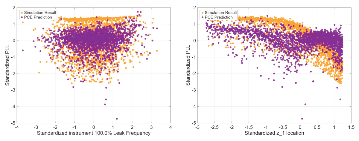
Figure 5
Comparison of the simulation results and regression results from the Case 1 single-loop analysis for the instrument rupture frequency (left) and z-location (right) versus the standardized PLL.
For the dual-loop analysis, a separate surrogate model was fit for each occupant location sample. Hence, the location parameters are no longer included in the surrogate model, but there is a separate surrogate model for each occupant location realization. Combining the results from these surrogate models (each model is applied only to the samples corresponding to its location realization), results in an estimate of the overall PLL. This empirical CDF is shown in Figure 6 for the PCE surrogate model. This shows much better agreement with the simulation results than the single loop analysis.
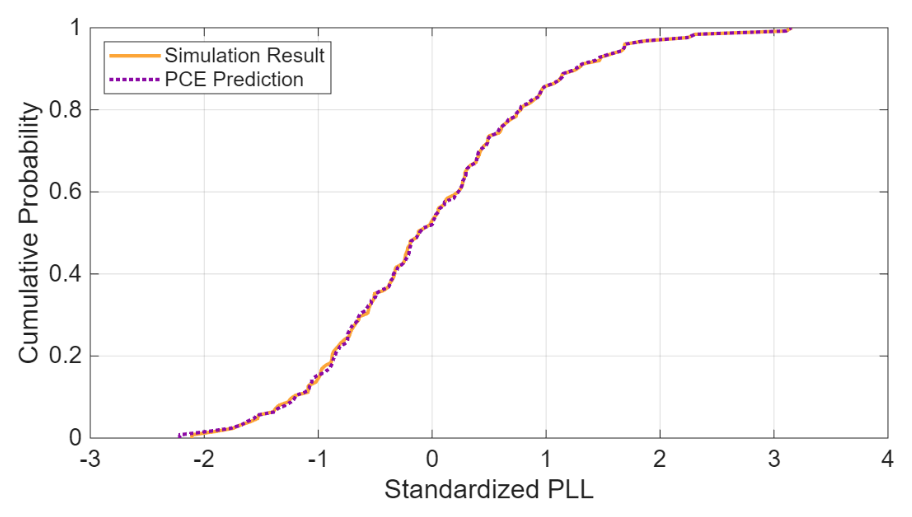
Figure 6
Comparison between the empirical cumulative distribution functions of the simulation results and the surrogate predictions for the Case 1 dual-loop analysis indicates a good fit in the regression analysis for PLL.
The scatterplots in Figure 7 help us understand why the surrogate performs much better in the dual-loop analysis. This plot shows the relationship between the instrument rupture frequency and the PLL (left) and between the joint rupture frequency and the PLL (right). The dual-loop surrogate results are colored in purple, and the QRA model results are colored in orange. The clusters of points in the scatterplot correspond to different samples of the occupant locations. Separate PCE models were fit for each cluster. This allows the within-cluster relationship between the rupture frequencies and the PLL to drive the surrogate model fit, whereas in the single-loop case, the variability due to occupant location and the variability due to instrument rupture frequency are not separable.
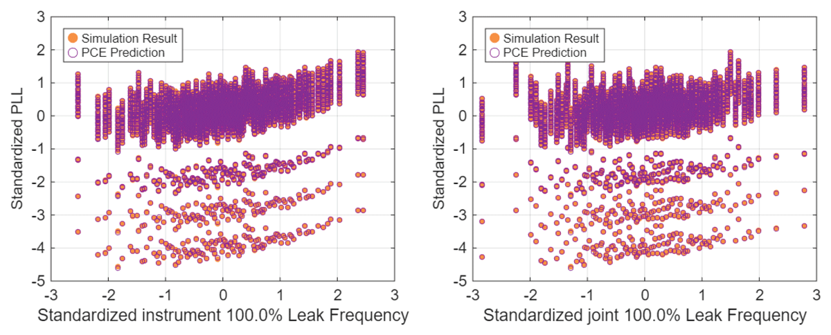
Figure 7
Comparison of the simulation results and regression results from the Case 1 dual-loop analysis for the standardized instrument rupture frequency (left) and standardized joint rupture frequency (right) versus the standardized PLL.
The total effect sensitivity indices from the PCE models fitted at each location sample in the dual-loop analysis are shown in Figure 8; the points are colored differently for each location. However, the coefficients are indistinguishable across the different regression models. It is clear that the instrument rupture frequency dominates uncertainty in the risk estimate. There is a secondary, lesser effect, from the joint rupture frequency. This is consistent with the plots in Figure 7; there is a slight positive trend with respect to joint rupture frequency and a much stronger positive trend with respect to instrument rupture frequency. Identification of inputs to which risk is sensitive can be helpful to inform decision-makers on where additional focus may be the most impactful, such as through additional data gathering or design changes.
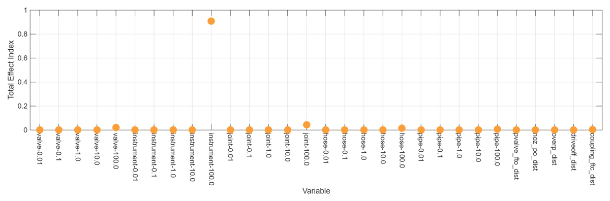
Figure 8
Total effect sensitivity indices for the Case 1 dual-loop analysis.
Cases 2, 3, and 4
The clear significance of rupture contributions to risk compared to smaller leaks could be a surprising result considering that smaller leaks are generally more common for most component types. To investigate this result further, additional cases were defined for SA, as discussed in the Methods section. Single- and dual-loop analyses were performed for Cases 2–4. However, the single-loop results were all similar to Case 1 (i.e., dominated by location), so only dual-loop results are shown here.
The dual-loop sensitivity results for Case 2 are shown in Figure 9. This case is the same as Case 1 except the occupants are moved closer to the leaks. The Case 2 SA differs from Case 1 in that the GP surrogate model performed better than PCE. The SA results from this GP are similar to Case 1, though there is more variation between location realizations, and there are some realizations in which pipe ruptures or valve ruptures contribute more to variation in the PLL than joint ruptures. This variation cannot definitively be attributed solely to the occupants being closer to the leaks. The PCE surrogate for Case 1 produces analytical estimates of the sensitivity indices, whereas the GP surrogate for Case 2 has to be sampled to estimate the sensitivity indices. Variability between indices in Case 2 may include some sampling uncertainty. However, it also makes sense that ruptures would dominate PLL results for occupants close to the leak, so the competing importance of various component ruptures in the sensitivity index results is probably not solely due to sampling uncertainty. Increasing the sample size used to estimate the sensitivity indices also did not eliminate this variation, which suggests the variation is not sampling uncertainty.
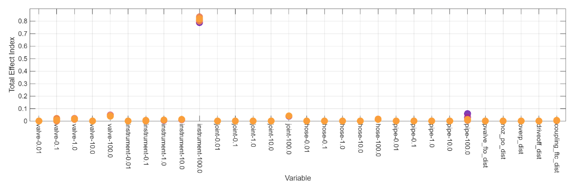
Figure 9
Total effect sensitivity indices for the Case 2 dual-loop analysis with different colors denoting different occupant location realizations.
The Case 3 analysis differed from Case 1 in that the system pressure was doubled. This change in the scenario did not result in significant differences in the SA results between Case 1 and Case 3. Hence, even in a higher-pressure system that increases the consequences associated with small leaks, the less frequent large-leak-size rupture events dominate risk. Additionally, the Case 3 SA was performed with a GP surrogate model. As in Case 1, the sensitivity indices are indistinguishable between location realizations, which would not be expected if the indices were affected by sampling uncertainty. For Case 3, there is no significant sampling uncertainty in the SA results. The same sample size was used for the GP surrogates in Case 2 and Case 3; the lack of significant sampling uncertainty for Case 3 further supports the argument that the variability between sensitivity results in Case 2 reflects true differences in the PLL between the location realizations, not sampling uncertainty. The Case 4 analysis included both the closer occupant locations from Case 2 and the higher pressure from Case 3. These results were very similar to the Case 2 results, reinforcing the conclusion that changing the system pressure did not change the relationship between input and output uncertainties. There is variation in the sensitivity indices in Case 4 as in Case 2, so there is evidence that moving the occupant locations closer to the leaks affects the relationship between some input uncertainties (rupture frequencies) and the output (PLL) uncertainty, regardless of system pressure.
Sensitivity analysis conclusions
Over the four sensitivity cases, the surrogate models performed better with a dual-loop sampling structure. The occupant location is the dominant uncertainty contributing to uncertainty in PLL and this relationship is not well-modeled by either a PCE or GP surrogate in the single-loop analysis. By fitting separate surrogate models to each location realization, the most significant non-location parameters contributing to uncertainty in the PLL were able to be identified. This separation of uncertainties was necessary to get good SA results.
Summary
QRA is a valuable tool for understanding the risks associated with specific system configurations and operating conditions of hydrogen systems. QRA will be needed to improve understanding of the risks associated with the increasing deployment of hydrogen technologies. Incorporation of UQ and SA methods will improve the effectiveness of QRA to inform safety decisions such as setback distances, necessary safety technologies, and system placement. Such methods can be readily incorporated into the QRA problems currently being solved using HyRAM+ to provide a more complete understanding of risk. Identification of sensitive inputs can be helpful to inform decision-makers on where additional focus may be the most impactful. For cases in which an input is highly uncertain due to a lack of data, obtaining more data through laboratory or operational records can help to reduce these uncertainties. Such studies can also be used to consider possible design changes to see if the resulting risk metrics show a significant risk reduction in comparison to these sources of uncertainty in the calculation.
With uncertainty, risk predictions spanned a range from around 10–12 to 10–4 fatalities per system-year, indicating substantial uncertainty around the deterministic estimate of 10–5.54. The median estimate from the UQ was found to be very close to the deterministic estimate. Uncertainty in the occupant location had the largest effect on uncertainty in PLL, but dual-loop analysis that separated occupant location from the other parameter uncertainties showed that leak frequencies for ruptures from instrumentation is the next most significant uncertainty. Depending on the simulation conditions, there may be a small effect on uncertainty in PLL from uncertainty in rupture frequencies for other components, such as joints, pipes, and valves. However, these effects are minor compared to the effect from the instrument rupture frequency.
An important note about the reported risk uncertainty and sensitivities is that they are specific to the system, conditions, and uncertainty distributions considered and that only a subset of all the uncertainty sources present in the calculations were accounted for in the results presented. Input distributions may reflect a lack of knowledge about the true value, but may also reflect variability in component types, maintenance differences, or human factors interactions. If additional sources of uncertainty were considered, the total uncertainty would likely increase, and the relative sensitivities might change. There can also be cases where the risk measure is most sensitive to one variable, but that is not the variable driving risk. This is why scatterplot analysis should always be included. For example, uncertainty in an input variable may drive the majority of the variation in PLL values for low-to-medium values of PLL but may have no influence on whether the PLL is high vs. low. Another variable may have no influence over variation in low-to-medium values of PLL but may wholly determine whether the PLL estimate is high. In a case like this, variance-based SA may identify the variable driving variation in low-to-medium PLL estimates as the most important, whereas the variable determining when PLL risk is high would be a better target for risk mitigation.
Applying UQ and SA methods to QRA calculations improved the understanding of the overall uncertainty in current risk estimates and those input uncertainties that contribute most to the uncertainty. The methods that were used are a significant advancement towards better informing risk decisions and establish a foundation from which the treatment of uncertainty with HyRAM+ can be improved.
Acknowledgements
The authors would like to thank Chris LaFleur, Kristin Hertz, and Marina Miletic of Sandia for their technical reviews of this paper.
Author Contributions
Dusty Brooks planned and performed the sensitivity analysis. Benjamin Schroeder set up the risk assessment and completed the uncertainty quantification analysis. Brian Ehrhart led the team and informed the direction of the studies. All authors contributed to writing and revision of the manuscript.