
Introduction
The adoption of hydrogen in the transport field aims to power vehicles without emitting greenhouse gases. Fuel cell electric vehicles (FCEVs), from light-duty (Toyota, 2024) to heavy-duty (Iveco, 2023) vehicles, can reach a similar range compared to their fossil-fuel counterparts with an equivalent refueling time.
The relatively low volumetric energy density of hydrogen must be enhanced to store it compactly for transport applications. A common solution is to compress the hydrogen in a gaseous form up to 700 bar to obtain a density of approximately 40 kg/m3 at a standard temperature of 15°C.
To reach 700 bar inside the compressed hydrogen storage system (CHSS), the refueling process requires managing the increase in the gas temperature inside the CHSS due to the compression. This is performed by selecting a refueling time and a fuel delivery temperature adapted to the refueling conditions (ambient temperature, precooling capacity, CHSS volume, etc.). This is the purpose of a refueling protocol.
Alongside standardization organizations, in particular the Society of Automotive Engineers (SAE), recommend safety guidelines during refueling (e.g., not to exceed 85°C in the gas (SAE International, 2020)).
Since 2023, the focus has been shifting from light-duty (SAE International, 2020) (<10 kg) to heavy-duty vehicles (>10 kg) (SAE International, 2023; SAE International, 2024a). Hence, trucks were the fastest-growing category of FCEVs (IEA, 2024). The CHSS capacity of the FCEVs is then expanded with trucks reaching 1750 L of total CHSS volume (Iveco, 2023).
The CHSS volume is an input for the two refueling protocols described in the SAE J2601 (SAE International, 2020): the MC method formula and the look-up tables. According to the CHSS volume, the average pressure ramp rate (APRR) and end-of-fill dispenser pressure differ.
The SAE J2601 (SAE International, 2020) classifies vehicle CHSS into four categories: A, B, C and D. Table 1 presents the different categories in the SAE. The technical information report (TIR) 5 of the SAE J2601 (SAE International, 2024a) adds subcategories to category D.
Table 1
Different tank categories in the SAE J2601.
| PRESSURE CLASS | WATER VOLUME OF CHSS (L) | CHSS CAPACITY CATEGORY |
|---|---|---|
| H35 | 49.7–99.4 | A |
| H35 | 99.4–174 | B |
| H35 | 174–248.6 | C |
| H70 | 49.7–99.4 | A |
| H70 | 99.4–174 | B |
| H70 | 174–248.6 | C |
| H70 | >248.6 | D |
[i] Abbreviation: CHSS: compressed hydrogen storage system.
Adapted from Table 8 from SAE International (2020).
The CHSS volume is a priori unknown when an FCEV reaches a hydrogen refueling station (HRS). However, the CHSS volume can be transmitted from the FCEV to the HRS, as specified in the SAE J2799 standard (SAE International, 2024b).
In the absence of communication, the HRS should estimate the CHSS volume. The SAE J2601 standard (SAE International, 2020) specifies that the startup time, which includes a connection pulse step for measuring the initial tank pressure, may also include a step for CHSS volume estimation. However, this startup time must be performed with <200 g of hydrogen.
For SAE refueling protocols, if the HRS cannot estimate the CHSS volumes within a ±15% error range or if the CHSS volume is indeterminate, the HRS should use the most conservative values, which implies the slowest APRR and the smallest end-of-fill dispenser pressure from the different CHSS capacity categories (SAE International, 2020; Appendix G). This impacts the refueling performance with a slower refueling time and a smaller final state of charge (SOC).
The consequence of using an incorrect CHSS category to select the APRR is not addressed in the SAE. On this matter, the risk assessment conclusion from the European project PRHYDE (Glatz et al., 2021) reports that inaccurate transmitted data must be addressed in refueling protocol risk assessments. Plausible scenarios that might lead to a discrepancy between the transmitted CHSS volume and the actual CHSS volume include part of the CHSS remaining closed, illegal CHSS modification, erroneous transmitted data, etc.
As a result, a method to estimate the CHSS volume shall be applied by the HRS during the earlier stage of the refueling, whether data are transmitted by the FCEV or not. The method shall be precise in accordance with the ±15% error range and be applicable regardless of the CHSS volume to be estimated.
Motivation
This study investigates two stages of CHSS volume estimation method: (i) the refueling step (i.e., the HRS’s data acquisition through physical measurements) followed by (ii) the volume estimation step (i.e., the development and application of mathematical formulations for volume estimation).
Refueling step
Yamaguchi et al. (2018) point out that for volumes larger than 100 L, 200 g of hydrogen injected might not be enough to perform a precise volume estimation during the startup time.
They suggested a method for the HRS to perform a CHSS volume estimation after the startup time to respect the 200 g injected mass criterion from SAE J2601 (SAE International, 2020). The SAE J2601-5 standard (SAE International, 2024a) adapted the work of Yamaguchi et al. (2018) to suggest a similar method.
If we consider a simplified HRS piping and instrumentation diagram (P&ID), shown in Figure 1, a control valve is located upstream of the dispenser. The piping system located between the dispenser and the CHSS (breakaway, hose, nozzle, etc.) is assimilated into an equivalent virtual valve in terms of head losses. Lastly, the CHSS volume is considered a single tank to simplify the following development.
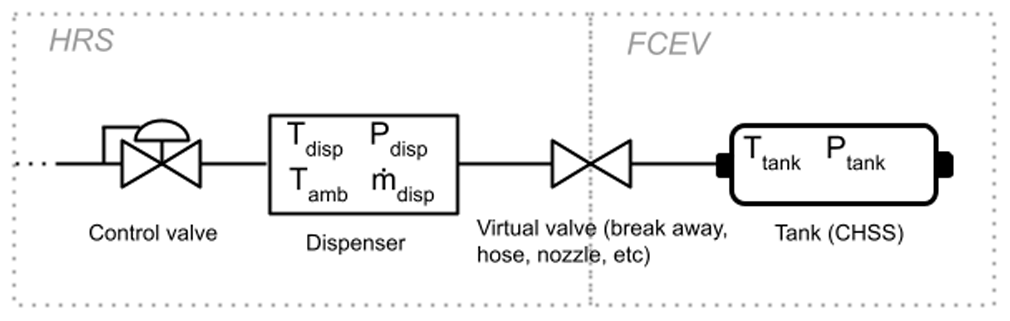
Figure 1
Simplified P&ID of the HRS section between the control valve and the CHSS of the FCEV. The data measured by the dispenser and transmitted by the FCEV are reported in the figure.
Abbreviations: CHSS: compressed hydrogen storage system; FCEV: fuel cell electric vehicle; HRS: hydrogen refueling station; P&ID: piping and instrumentation diagram.
At the dispenser, the pressure Pdisp (MPa (g)), temperature Tdisp (°C) and mass flow rate (kg/s) of the refueling flow are measured continuously. Likewise, the ambient temperature Tamb (°C) is measured by the HRS.
After the connection pulse, the control valve is closed, and the pressure of the gas in the dispenser Pdisp (MPa) equalizes the pressure of the gas in the tank Ptank (MPa). This moment is noted t0 (s), then,
To estimate a tank volume, the intent is to raise the pressure in the tank. The tank pressure elevation ΔPtank (MPa) must be sufficient to be accurately measured by a pressure sensor. In the SAE J2601-5 (SAE International, 2024a), a pressure elevation of 5 MPa is targeted.
To get a pressure elevation ΔPtank in the tank, a refueling step is required. To ensure safety, the refueling uses a conservative APRR.
Due to the head losses between the dispenser and the tank, the pressure in the tank is lower than the pressure at the dispenser. Consequently, to reach a targeted pressure elevation ΔPtank [MPa] in the tank, a pressure overshoot ΔPdisp (MPa) is targeted at the dispenser.
In the SAE J2601-5 (SAE International, 2024a), this overshoot is expressed as a function of the initial pressure Ptank(t0) (MPa), such as for a refueling up to 700 bar (H70),
In the study, only H70 refueling will be considered. Accordingly, equation (2) will be employed to calculate the dispenser overshoot pressure elevation.
The refueling step ends when the dispenser reaches the pressure Pdisp(t0) + ΔPdisp. Then, the pressure in the dispenser drops and equalizes the pressure in the tank. This moment is noted t1 [s], then
and finally,
The injected mass Δm (kg) in the tank is obtained via a numerical integration of the mass flow rate (kg/s) measured at the dispenser,
These refueling steps must be considered independently of the volume estimation calculation. A primary purpose of this study is to verify that the refueling step suggested by the SAE J2601-5 allows for an exploitable pressure tank elevation ΔPtank and injected mass Δm.
Hence, once a pressure tank elevation ΔPtank and injected mass Δm are obtained, the method to calculate the tank volume V (m3) differs depending on how the temperature in the tank is calculated.
Volume estimation step
Let us consider the hydrogen in the tank as a uniform region, that is, 0-dimensional (0D) modeling. The mass in the tank can be expressed as
where ρ (kg/m3) is the density of hydrogen and Ttank (°C) is the temperature inside the tank. During the refueling step, the density and the mass vary, but the volume remains constant. This leads to
Then the evaluation of the volume depends on the evaluation of Ttank(t0) and Ttank(t1), which are unknown in the absence of communication between the HRS and the FCEV.
For Yamaguchi et al. (2018) and in the standard SAE J2601-5 (SAE International, 2024a), the initial tank temperature Ttank(t0) is considered equal to the ambient temperature, that is,
This assumption is also made in this study. However, additional studies could be carried out to investigate the impact of the initial gas temperature estimation on the volume estimation, using, for instance, the hot/cold soak concept from the SAE J2601 (SAE International, 2020).
Due to the pressure elevation inside the tank, the temperature also increases, that is, Ttank (t1) > Ttank(t0). However, an estimation of Ttank(t1) is dependent on several factors such as the tank geometry (aspect ratio) and materials (tank type III, IV, etc.). It also depends on the refueling time, which can vary largely according to the ambient temperature and the precooling capacity of the HRS.
A secondary purpose of this study is to introduce different volume estimation formulations constructed from different physical hypotheses. From experimental data of refueling using different initial pressures and fuel delivery temperatures, the volume calculated from these formulations will be compared and discussed.
Physical Modeling
This section aims to detail the different formulations that can be used to evaluate the CHSS volume of an FCEV.
They are based on a thermodynamic model of the gas in the tank, that is, 0D modeling (Bourgeois et al., 2015; Kuroki et al., 2021; Molkov et al., 2019). Hence, the governing gas equations are the mass (9) and energy balance equations (10). To simplify the notation, physical parameters concerning the gas inside the tank are noted without the ‘tank’ index (e.g., Ttank → T; Ptank → P). Then,
where m (kg) is the internal gas mass, T (K) is the internal gas temperature, P (Pa) is the internal gas pressure, V (m3) is the tank volume, β (1/K) is the isochoric expansion coefficient, cp (J/kg/K) is the specific gas heat capacity, h (J/kg) is the specific enthalpy of the hydrogen, Tinj (K) is the injection temperature and uinj (m/s) is the injection gas velocity.
The term kgSw,int(Tg,w – T) models the heat exchanged with the walls, where Tg,w (K) is the internal tank wall temperature, Sw,int (m2) is the internal tank wall surface in contact with the gas and kg (W/m2/K) is the heat transfer coefficient between the gas and the walls.
Gas properties, for example, gas density and enthalpy, are functions of the tank pressure and temperature. These functions are assumed to be known. They can be evaluated via gas property libraries based on the National Institute of Standards and Technology (NIST) data, such as CoolProp (Bell et al., 2014), REFPROP (Lemmon et al., 2018) or via polynomial regression functions (Park and Chae, 2021). In this study, gas properties are evaluated with CoolProp.
Applying a differential approximation of the gas mass variation can be an approach to evaluate the volume. Hence, considering the mass in the tank equation (6), an infinitesimal mass variation can be expressed as
Then, a first-order approximation of the mass variation is
SAE J2601-5 formulation
The volume estimation formulation defined in the standard SAE J2601-5 (SAE International, 2024a) introduces measurement accuracy for the dispenser pressure sensor Ptol (MPa) and for the mass flow rate sensor mtol (%).
Then, the initial gas density is calculated as
The final gas density is calculated using a temperature elevation ΔTSAE (°C) in the tank, a function of the initial pressure Ptank(t0) (MPa). Hence, for H70 refueling,
Then,
The CHSS volume is calculated as
It must be noted that in the SAE, the dispenser pressure tolerance and mass flow rate measurement tolerance are used to overestimate the volume. This is a conservative approach, that is, it prevents over-temperature events in the tank for SAE refueling protocols. Hence, estimating a larger CHSS volume implies a slower refueling ramp and final pressure, thus a smaller temperature elevation inside the tank.
However, this approach can be non-conservative regarding overfilling when refueling control is based on the mass flow rate. For instance, if we consider calculating the SOC for a given nominal working pressure (NWP), PNWP (MPa) and using the mass flow rate,
An overestimated CHSS volume leads to an underestimated SOC. If the refueling control is based on this SOC, a tank overfilling event could occur. For this application, the conservative approach is to underestimate the CHSS volume. Consequently, a conservative approach depends on the event to prevent, for example, overfilling, over-temperature, and the refueling control chosen, for example, pressure ramp rate or mass flow rate.
Isothermal formulation
A simple formulation can be obtained by neglecting the temperature elevation inside the tank, that is, Ttank(t1) = Ttank(t0).
This hypothesis implies that the heat transferred from the gas to the walls is sufficient to maintain the temperature almost constant. This can correspond to a very slow refueling.
Because the temperature elevation inside the tank is underestimated, this formulation tends to underestimate the CHSS volume. Using equation (7), the volume can be calculated directly.
Using the first-order (FO) approximation of the mass variation from equation (12), it can be shown that
with evaluated at the initial time t0.
The discrepancy between equations (18) and (19) is interesting to evaluate the error made by the first-order approximation of the mass variation. It should be noted that the subsequent adiabatic and diabatic formulations will also utilize a first-order approximation, but the suffix ‘FO’ will be omitted from the method names for simplicity.
Adiabatic formulation
Another formulation can be obtained by neglecting the heat transferred from the gas to the walls. This implies kgSw,int(Tg,w – T) = 0. This hypothesis can correspond to a very fast refueling.
The impact of the kinetic energy on the gas temperature is considered negligible for a short time period.
The enthalpy injected in the tank h(P, Tinj) must be evaluated. A hot dispenser hypothesis is assumed, that is, h(P, Tinj) = h(P, Tamb).
These hypotheses tend to overestimate the temperature elevation inside the tank and, consequently, the CHSS volume. From equations (10) and (12), it can be shown that
with evaluated at the initial time t0.
Diabatic formulation
During the refueling step, the gas inside the tank exchanges heat with the walls. This phenomenon is influenced by the refueling time. Moreover, according to the ambient temperature, the refueling step can vary largely.
For instance, let us consider a refueling with no communication and a fuel delivery temperature of –30°C. The initial measured tank pressure is Ptank = 2 MPa(g). This implies, using equation (2), that ΔPdisp = 12.33 MPa.
According to the conservative table G4 from SAE J2601-5 (SAE International, 2024a), at Tamb = 0°C, the APRR = 22 MPa/min and at Tamb = 30°C, the APRR = 7.5 MPa/min. Then, at Tamb = 0°C, a refueling step takes approximately 30 s while at Tamb = 30°C, it takes approximately 100 s.
Accordingly, a volume estimation formulation should take into account the refueling time of the refueling step.
Estimating the heat transferred from the gas to the walls is challenging. This could be performed with a 0D modeling simulation but requires knowing the geometry and the materials of the tank and the piping. Due to the absence of such information, several assumptions have to be made. Notably, the CHSS volume is an input for a 0D modeling simulation.
To address this challenge, two methods are developed in this section. The first one is a direct method, comparable with the isothermal and adiabatic formulations. The CHSS volume is directly calculated from the data collected at times t0 and t1. Despite requiring approximations, this method is suitable to be implemented into the programmable logic controller (PLC) of HRS.
The second method is an iterative approach. It uses a dichotomy algorithm along with a 0D modeling simulation and an initial CHSS volume guess to converge toward a precise CHSS volume.
Direct method
Like the adiabatic method, the effect of the kinetic energy on the gas temperature is neglected. The injected gas temperature Tinj is taken as the mass-averaged temperature from the dispenser temperature:
This corresponds to a cold dispenser. From the energy balance equation (10), it can be shown that
The quantity (T – Tg,w) is approximated by
The quantity depends on the aspect ratio of the tank. The quantity kg depends on several parameters (Woodfield et al., 2007) (e.g., the tank and injector geometry, the injection velocity, the buoyancy forces, etc.). The product is here considered constant during the refueling step and noted Λ (W/m3/K), that is, . This leads to
Another form of equation (11) is
By substituting equation (24) into equation (25), it can be shown that
Considering , it can be shown that,
Then, considering all thermophysical properties calculated at t0, it can be shown that
It must be noted that if Δt → 0, then Vdia → Vadia, and if Δt → +∞, then Vdia → Viso. The parameter Λ controls the transition rate between the two formulas. Depending on whether an overestimation or an underestimation of the CHSS volume is needed, the parameter Λ shall be adjusted.
For example, a configuration that leads to an underestimate of the heat transferred from the gas to the walls tends to overestimate the CHSS volume. This configuration is selected in this study by using the smallest surface-to-volume ratio from tank geometry assumptions from SAE J2601-5 (SAE International, 2024a), m–1. A limited heat transfer coefficient is selected, likewise the one found for the slow refueling case issued from Monde et al. (2012), kg = 45 W/m2/K. Finally, Λ = 303 W/m3/K.
The flowchart of the diabatic formulation is detailed in Figure 2.
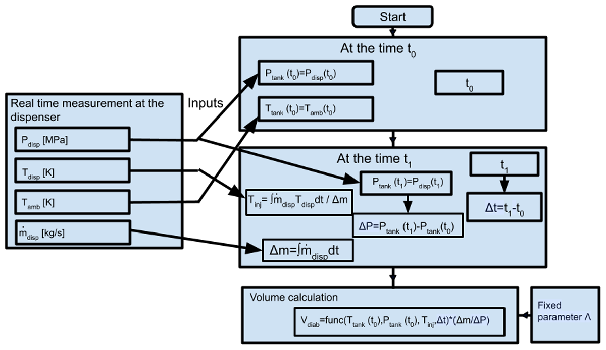
Figure 2
Flowchart of the diabatic formulation.
Direct method approximated
The diabatic volume estimation is interesting for practical applications because its direct evaluation requires a limited number of operations. A PLC shall have the computation resource to perform a calculation.
However, equation (28) requires hydrogen thermophysical properties to be evaluated. To allow rapid evaluation of equation (28), a polynomial approximation method is developed.
Let us consider the approximated diabatic formula Vdia–approx (m3).
Let us define the effective volumetric thermal capacity Ccp–eff (J/m3/K):
the non-dimensional time τ (no unit):
and a transition function F:
It can be shown that
considering
The coefficient Ciso(P, T), Cadia(P, T, Tinj) and Ccp–eff(P, T) can be evaluated using polynomial functions. The polynomial regression is performed for T ∈ [–40°C, 85°C], Tinj ∈ [–40°C, 50°C] and P ∈ [0.5 MPa(g), 87.5 MPa(g)]. Table 2 presents the coefficients for fifth-order polynomial functions. The coefficient is associated with the polynomial term (e.g., 1, Tinj, Tinj2, etc).
Table 2
Coefficient table for the polynomial functions Ciso(P, T), Cadia(P, T, Tinj) and Ccp–eff(P, T).
| TERM | Ciso COEFFS | Cp-eff COEFFS | Cadia COEFFS |
|---|---|---|---|
| 1 | 1.1283600E+06 | 8.0916516E+02 | 1.5907225E+06 |
| Tinj | 0.0000000E+00 | 0.0000000E+00 | 5.8152799E+03 |
| Tinj2 | 0.0000000E+00 | 0.0000000E+00 | 1.0473866E+00 |
| Tinj3 | 0.0000000E+00 | 0.0000000E+00 | –4.3391871E–03 |
| Tinj4 | 0.0000000E+00 | 0.0000000E+00 | 8.6699560E–06 |
| Tinj5 | 0.0000000E+00 | 0.0000000E+00 | –2.4108136E–08 |
| T | 4.1345584E+03 | –2.1782544E–01 | –2.2584316E+02 |
| T*Tinj | 0.0000000E+00 | 0.0000000E+00 | –2.9014440E+00 |
| T*Tinj2 | 0.0000000E+00 | 0.0000000E+00 | –5.9850516E–04 |
| T*Tinj3 | 0.0000000E+00 | 0.0000000E+00 | 2.8617328E–06 |
| T*Tinj4 | 0.0000000E+00 | 0.0000000E+00 | –1.9133298E–08 |
| T2 | –3.9128813E–01 | 4.5885629E–02 | 2.3204987E+00 |
| T2*Tinj | 0.0000000E+00 | 0.0000000E+00 | 2.6318857E–02 |
| T2*Tinj2 | 0.0000000E+00 | 0.0000000E+00 | 3.2417329E–06 |
| T2*Tinj3 | 0.0000000E+00 | 0.0000000E+00 | –2.6388874E–08 |
| T3 | 4.8869951E–03 | –1.0613305E–03 | –1.9312110E–02 |
| T3*Tinj | 0.0000000E+00 | 0.0000000E+00 | –2.0154968E–04 |
| T3*Tinj2 | 0.0000000E+00 | 0.0000000E+00 | –9.3200198E–09 |
| T4 | 1.0076258E–06 | 3.0320051E–06 | 2.1059983E–04 |
| T4*Tinj | 0.0000000E+00 | 0.0000000E+00 | 8.5624925E–07 |
| T5 | –1.6012029E–07 | 2.1608048E–08 | –1.0304455E–06 |
| P | 1.3614112E+04 | 8.9668248E+03 | 2.1697410E+04 |
| P*Tinj | 0.0000000E+00 | 0.0000000E+00 | 6.3710870E+01 |
| P*Tinj2 | 0.0000000E+00 | 0.0000000E+00 | –4.5069595E–02 |
| P*Tinj3 | 0.0000000E+00 | 0.0000000E+00 | 5.2637944E–05 |
| P*Tinj4 | 0.0000000E+00 | 0.0000000E+00 | 1.5242998E–07 |
| P*T | 2.2820956E+01 | –2.9038600E+01 | –5.3663267E+01 |
| P*T*Tinj | 0.0000000E+00 | 0.0000000E+00 | –2.7913640E–01 |
| P*T*Tinj2 | 0.0000000E+00 | 0.0000000E+00 | 1.0626895E–05 |
| P*T*Tinj3 | 0.0000000E+00 | 0.0000000E+00 | 8.8698092E–08 |
| P*T2 | –5.4810045E–02 | 6.9133477E–02 | 3.4922958E–01 |
| P*T2*Tinj | 0.0000000E+00 | 0.0000000E+00 | 1.2330859E–03 |
| P*T2*Tinj2 | 0.0000000E+00 | 0.0000000E+00 | –4.7593259E–09 |
| P*T3 | –3.0271457E–04 | –2.8540368E–05 | –1.9932921E–03 |
| P*T3*Tinj | 0.0000000E+00 | 0.0000000E+00 | –2.3767989E–06 |
| P*T4 | 1.3146260E–06 | –2.6105553E–07 | 4.1096764E–06 |
| P2 | 1.6414600E+02 | –5.0523257E+01 | 1.8501464E+02 |
| P2*Tinj | 0.0000000E+00 | 0.0000000E+00 | –3.4170773E–01 |
| P2*Tinj2 | 0.0000000E+00 | 0.0000000E+00 | 7.5245467E–04 |
| P2*Tinj3 | 0.0000000E+00 | 0.0000000E+00 | –9.1746565E–07 |
| P2*T | –1.0389051E+00 | 3.1786849E–01 | –8.8709648E–01 |
| P2*T*Tinj | 0.0000000E+00 | 0.0000000E+00 | 1.3000849E–03 |
| P2*T*Tinj2 | 0.0000000E+00 | 0.0000000E+00 | –1.4771480E–07 |
| P2*T2 | 3.2574499E–03 | –1.0656155E–03 | 1.5205511E–03 |
| P2*T2*Tinj | 0.0000000E+00 | 0.0000000E+00 | –5.3952236E–06 |
| P2*T3 | –1.8807052E–06 | 1.0760745E–06 | 5.8572045E–06 |
| P3 | –1.5591316E+00 | 1.9073393E–01 | –1.9570425E+00 |
| P3*Tinj | 0.0000000E+00 | 0.0000000E+00 | 1.3755835E–03 |
| P3*Tinj2 | 0.0000000E+00 | 0.0000000E+00 | –3.6679280E–06 |
| P3*T | 8.2229225E–03 | –1.6978191E–03 | 9.6192507E–03 |
| P3*T*Tinj | 0.0000000E+00 | 0.0000000E+00 | –1.1676633E–06 |
| P3*T2 | –1.7633706E–05 | 4.5014322E–06 | –1.8160604E–05 |
| P4 | 9.6056237E–03 | 8.2909304E–05 | 1.2227065E–02 |
| P4*Tinj | 0.0000000E+00 | 0.0000000E+00 | –2.6843097E–06 |
| P4*T | –2.4421704E–05 | 3.2439269E–06 | –3.1950194E–05 |
| P5 | –2.7419060E–05 | –2.6875205E–06 | –3.4507177E–05 |
Iterative method
If the PLC has sufficient computational resources to perform a 0D modeling simulation, an iterative approach can be performed to increase the precision.
A 0D modeling simulation is solving the mass and energy equations (9) and (10) using as inputs data from the dispenser, and producing, as outputs, the pressure and temperature inside the tank. As previously stated, it requires knowing the geometry and the materials of the tank and the piping.
In this study, a dichotomy approach is selected. The isothermal method estimates a minimum CHSS volume, while the adiabatic method estimates a maximum CHSS volume. This sets the CHSS volume interval in which the dichotomy method searches for an optimal volume. The initial guess is taken as the middle of this interval.
For a given CHSS volume, the 0D modeling simulation is calculating a pressure inside the tank Ptank–calc(t) as a function of time. At time t1, the calculated pressure Ptank–calc(t1) is compared to the measured pressure Ptank(t1). (i) If superior, this means the selected CHSS volume is underestimated. The search interval is then reduced using the selected CHSS volume as the new lower bound. (ii) If inferior, this means the selected CHSS volume is overestimated. The search interval is then reduced using the selected CHSS volume as the new upper bound. Figure 3 shows the flowchart of the method.
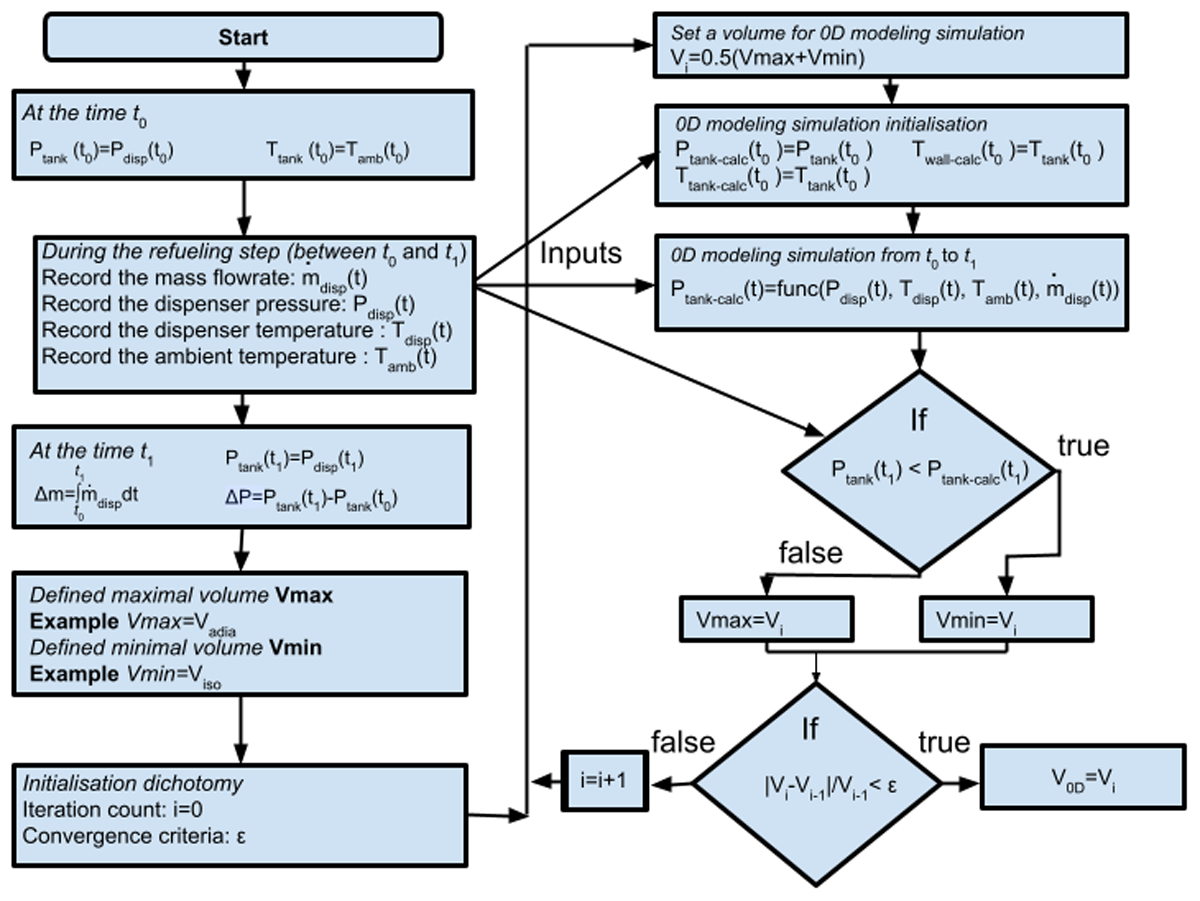
Figure 3
Flowchart of the iterative method.
According to the selected geometry and materials of the tank and the piping (e.g., hot case or cold case), the CHSS volume will tend to be overestimated or underestimated, respectively.
In this study, the influence of the tank and the dispenser is investigated by selecting:
A hot case tank and a cold dispenser V0D–HotCaseCD constructed from the tank from SAE J2601-5 (SAE International, 2024a) (geometry from Table A7, material properties from Table A11) and assuming hinj = h(Pdisp, Tdisp).
A hot case tank and a hot dispenser V0D–HotCaseHD constructed from the same previous tank and a dispenser from SAE J2601-5 (SAE International, 2024a) (piping geometry and materials from Tables A17–A21).
A cold case tank and a cold dispenser V0D–ColdCaseCD constructed from the tank from SAE J2601 (SAE International, 2020) (geometry from Table A3, 70 MPa, Type III) and assuming hinj = h(Pdisp, Tdisp).
Experimental Tests
Field testing cases are carried out at an experimental facility located at the Air Liquide Innovation Campus Delaware. Two tanks are selected: a type IV 243.6 L with an NWP of 700 bar and a type IV 1520 L with an NWP of 250 bar.
Both tanks are equipped with a thermocouple tree inserted in the rear region of the tank, opposite to the injector. From this thermocouple tree, an average gas temperature can be precisely extracted. Figure 4 presents the device used for the 243.6 L tank.
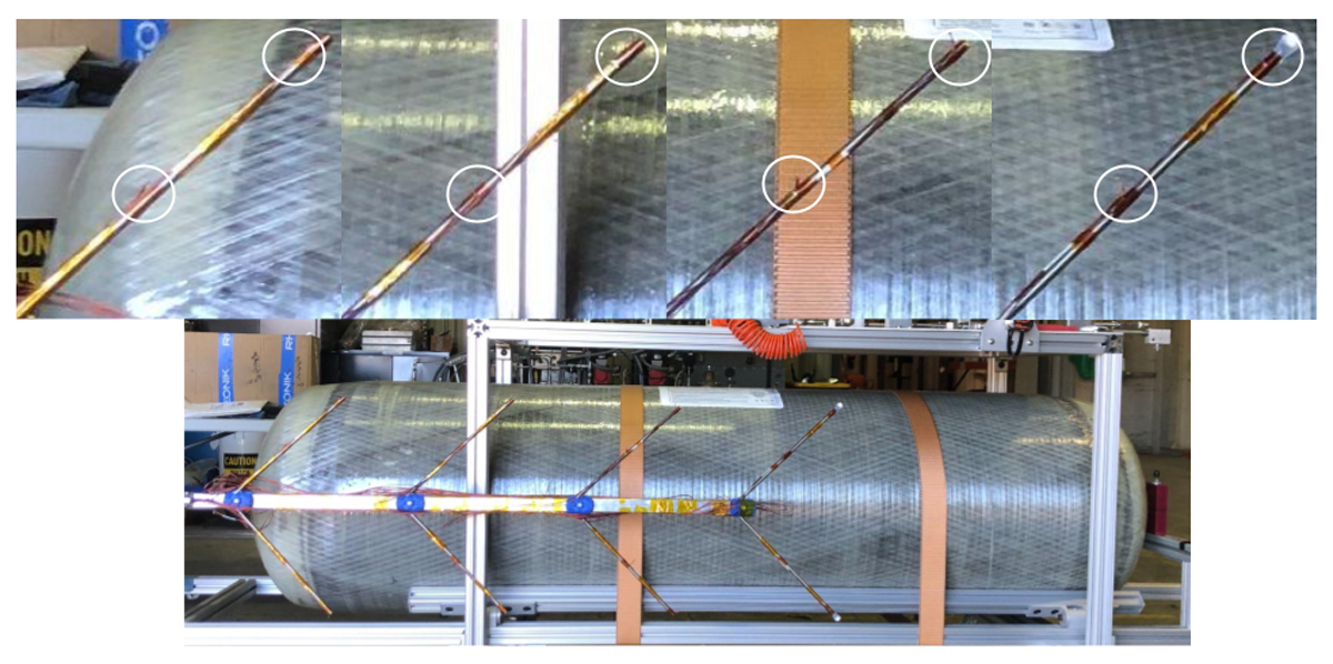
Figure 4
View of the 243.6 L thermocouple tree. It is placed in front of the tank for visualization but is then inserted inside the tank volume during the refueling tests. A zoomed view at the upper tank part highlights with white circles the presence of the thermocouple probes on the thermocouple tree branches. The thermocouple tree is symmetrical.
The experimental facility has some limits that must be specified:
The SAE J2601-5 (SAE International, 2024a) is not yet implemented; therefore, the look-up table category C (non-communications) from SAE J2601 (SAE International, 2020) is selected instead.
For the type IV 243.6 L tank tests, the PLC of the HRS could not be modified. To automatically stop the refueling at the targeted dispenser pressure, this is performed manually by an operator. This triggers an automatic safety purge in the line between the dispenser and the tank. The dispenser pressure rapidly falls to the atmospheric pressure. Then, at time t1, the tank pressure cannot be measured via the dispenser. The tank pressure is directly measured inside the tank using a pressure sensor located inside the tank.
The HRS has been designed for light-duty vehicles. The head loss of the piping system might differ from an HRS designed for heavy-duty vehicles. This could impact the pressure elevation inside the tank after the refueling step.
For the type IV 1520 L tests, it was not possible to physically stop the dispenser at the target pressure. To overcome this difficulty, data were collected continuously and then truncated once the target dispenser pressure was reached.
For the calculation, no tolerance corrections are applied to SAE equations (13), (15) and (16).
Type IV 243.6 L tank
The NWP of the 243.6 L tank allows investigating high initial pressures, and eight experimental refueling scenarios are considered involving different initial pressures (≈3, 11, 20, 31 MPa(g)) and different delivery temperatures (≈–20°C, –30°C). Note that due to the thermal inertia of the precooling system, the initial dispenser temperature at the very beginning of the injection is typically higher (e.g., around –10°C) before rapidly reaching the target delivery temperature.
Figure 5 presents the data issued from the mass flow rate, pressure and temperatures measured at the dispenser, and the pressure and average temperature measured in the tank.
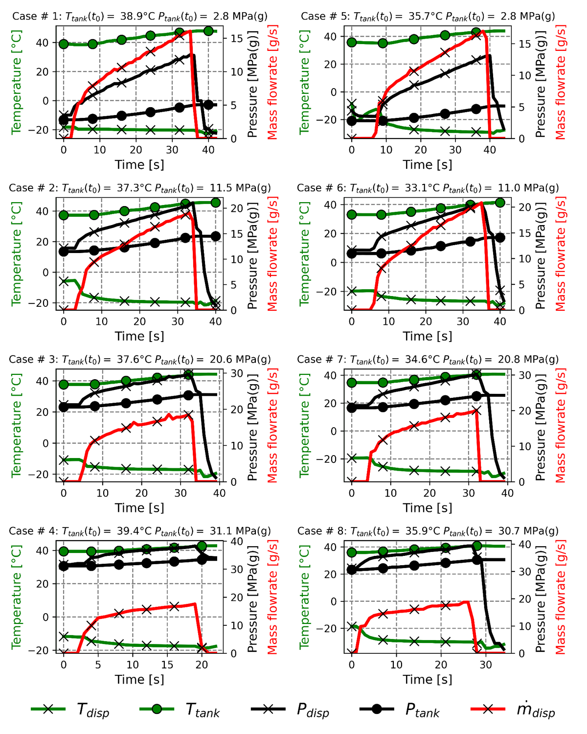
Figure 5
Plotting of the experimental data measured during the eight refueling steps of the type IV 243.6 L tank.
It can be seen that for all tests, the 5 MPa pressure elevation expected in the tank by SAE J2601-5 was never reached. The experimental pressure elevations in the tank are between 2.23 and 3.67 MPa (as detailed in Table 3), depending on the initial conditions of each case. This could be due to the head loss performance of the employed HRS.
Table 3
Numerical applications of the volume estimation formula based on the experimental data.
| TEST # | 1 | 2 | 3 | 4 | 5 | 6 | 7 | 8 |
|---|---|---|---|---|---|---|---|---|
| Ptank(t0) (MPa(g)) | 2.8 | 11.48 | 20.61 | 31.12 | 2.79 | 10.98 | 20.75 | 30.65 |
| Tamb(t0) (°C) | 29.15 | 30.59 | 30.4 | 30.77 | 27.79 | 28.41 | 29.18 | 31.36 |
| Tinj (°C) | –20.05 | –18.75 | –16.54 | –16.7 | –27.45 | –26.03 | –27.94 | –29.06 |
| Δt (s) | 37 | 35 | 34 | 21 | 40 | 37 | 33 | 28 |
| ΔPtank (MPa) | 2.23 | 2.99 | 3.43 | 2.38 | 2.34 | 3.08 | 3.5 | 3.67 |
| Δm (kg) | 0.38 | 0.42 | 0.43 | 0.25 | 0.39 | 0.45 | 0.44 | 0.41 |
| ΔTtank (°C) | 8.01 | 8.20 | 6.55 | 3.40 | 8.55 | 8.32 | 5.98 | 4.89 |
| ΔTSAE (°C) | 23.91 | 15.24 | 10.36 | 8.07 | 23.92 | 15.62 | 10.31 | 8.13 |
| Viso (L) Relative error % | 220.2 –9.6 | 206.4 ⚠ –15.3 | 203.7 ⚠ –16.4 | 192.0 ⚠ –21.2 | 218.5 –10.3 | 208.8 –14.3 | 206.4 ⚠ –15.3 | 202.4 ⚠ –16.9 |
| Viso–FO (L) Relative error % | 217.4 –10.8 | 202.9 ⚠ –16.7 | 199.8 ⚠ –18.0 | 189.5 ⚠ –22.2 | 215.5 –11.5 | 205.1 ⚠ –15.8 | 202.3 ⚠ –16.9 | 198.4 ⚠ –18.6 |
| Vadia (L) Relative error % | 305.7 ⚠ 25.5 | 287.0 ⚠ 17.8 | 283.4 ⚠ 16.3 | 268.8 10.3 | 303.2 ⚠ 24.5 | 290.2 ⚠ 19.1 | 287.1 ⚠ 17.9 | 281.4 ⚠ 15.5 |
| Vdia (L) Relative error % | 249.6 2.5 | 240.5 –1.3 | 242.1 –0.6 | 232.0 –4.8 | 242.1 –0.6 | 238.2 –2.2 | 236.7 –2.8 | 232.5 –4.6 |
| Vdia–approx (L) Relative error % | 252.7 3.7 | 239.2 –1.8 | 242.7 –0.4 | 231.6 –4.9 | 240.7 –1.2 | 240.8 –1.2 | 234.6 –3.7 | 234.9 –3.6 |
| V0D–hotCaseCD (L) Relative error % | 258.9 6.3 | 247 1.4 | 247.6 1.6 | 229.5 –5.8 | 253.1 3.9 | 245.6 0.8 | 242.8 –0.3 | 240.8 –1.2 |
| V0D–hotCaseHD (L) Relative error % | 292.4 ⚠ 20 | 280.5 ⚠ 15.1 | 278.1 14.2 | 260.4 6.9 | 291.8 ⚠ 19.8 | 283 ⚠ 16.2 | 280.1 ⚠ 15 | 279.3 14.7 |
| V0D–coldCaseCD (L) Relative error % | 240.9 –1.1 | 234 –3.9 | 234.6 –3.7 | 217.2 –10.8 | 238.3 –2.2 | 234.8 –3.6 | 232.3 –4.6 | 231.3 –5 |
| VSAE (L) Relative error % | 264.7 8.7 | 269.7 10.7 | 266.6 9.5 | 306.8 ⚠ 25.9 | 261.4 7.3 | 270.6 11.1 | 269.0 10.4 | 269.2 10.5 |
[i] Cells indicate the relative error below the volume value. Volumes with errors greater than 15% are reported with the symbol ⚠ (reference volume 243.6 L).
This default of pressure elevation induces a limited temperature elevation in the tank, below the one calculated using SAE temperature correlation; see equation (14).
This highlights that SAE temperature correlation cannot be used if the pressure elevation in the tank does not reach the 5 MPa expected value.
It can be seen that the initial tank temperature is always higher than the ambient temperature. This can be explained by the effect of the initial pulse test on the gas temperature. Hence, the pulse test consists of injecting a small amount of gas inside the tank, triggering a check valve opening and immediately stopping the mass flow rate. If the HRS is not sufficiently reactive, that is, more hydrogen mass than necessary is injected inside the tank, this step raises the gas pressure and temperature. That is what happened during the experimental tests.
Finally, it can be noted that the ambient temperature was relatively constant with values between 27.61°C and 30.7°C. The initial gas temperatures were between 33°C and 39.9°C. The effect of the initial temperature cannot be considered well covered by these tests.
Type IV 1520 L tank
The type IV 1520 L tank is designed for hydrogen ferries. This tank volume is characteristic of a heavy-duty storage system. This aspect motivates using it to investigate the volume estimation methods. However, its NWP is only 250 bar, and this limits higher-pressure investigations.
For NWP of 250 bar, the hydrogen test bench employed was able to test custom pressure ramps and injection temperature. Accordingly, two tests were performed out of the refueling step defined in the SAE J2601-5 (SAE International, 2024a): a slow one (refueling step during 935 s) and using a less precooling (–5°C) and a fast one (refueling step of 22 s) using the maximum precooling of the station (–30°C).
A total of six experimental refueling scenarios are considered involving different initial pressures (≈2, 10 MPa(g)), different temperatures of injection (≈–5°C, –20°C, –30°C) and different refueling times. Figure 6 presents the data issued from the mass flow rate, pressure and temperatures measured at the dispenser and the pressure and average temperature measured in the tank.
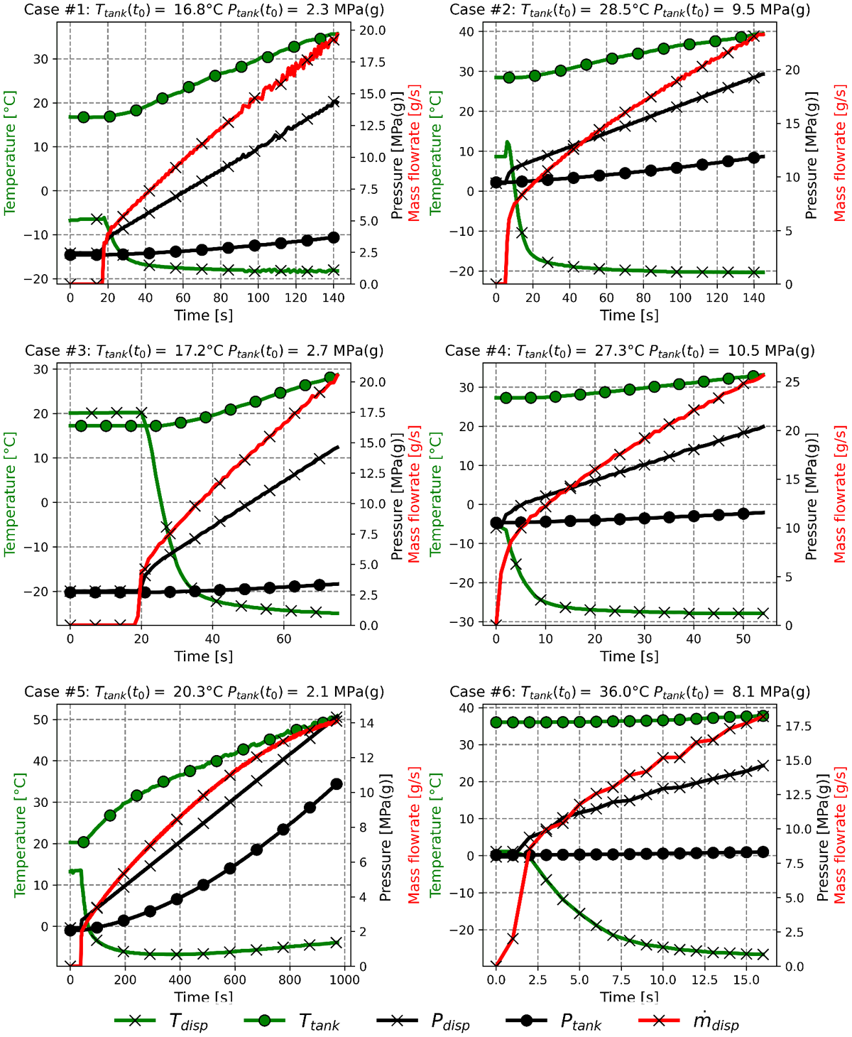
Figure 6
Plotting of the experimental data measured during the six refueling steps of the type IV 1520 L tank.
For the type IV 1520 L tank, during cases 1–4 using the APRR from the table-based protocol, the expected pressure elevation of 5 MPa was never reached. The same observation applies to case 6, using a faster APRR than table-based protocols.
Pressure elevations in the tank are very small, between 0.25 and 2.42 MPa. This is not sufficient to ensure precise pressure measurements. These results can be explained by the large pressure drop at the dispenser caused by the large mass flow rate (20 g/s) and small injector diameter (5 mm) employed.
Only test 5, using a slow APRR, outperformed 5 MPa and reached 8 MPa. Indeed, by using a slow APRR, the mass flow rate is reduced. Consequently, the pressure drop between the dispenser and the tank is reduced. Then, overshooting the dispenser pressure to ensure a pressure elevation for a given pressure drop within an HRS in the tank leads to overshooting the pressure elevation in the tank when the real pressure drop is lower. Exceeding a pressure elevation of 5 MPa induces a gas temperature elevation (ΔTtank = 30.51°C) superior to the one expected by the SAE (ΔTSAE = 24.87°C).
Compared to 243.6 L tank tests, initial gas temperatures are less affected by the pulse test. This can be explained by the large volume capacity. Hence, this limits the gas temperature elevation for the same amount of mass used during the pulse test.
Finally, it can be noted that the ambient temperatures are more diverse compared to 243.6 L tank tests, with values between 12.78°C and 25.58°C.
Results and Discussion
In this section, for the two tanks, a numerical application is performed on the different volume estimation formulations: VSAE (equation 16), Viso (equation 18), Viso–FO (equation 19), Vadia (equation 20), Vdia (equation 28), Vdia–approx (equation 32), V0D–HotCaseCD, V0D–HotCaseHD, and V0D–ColdCaseCD.
Type IV 243.6 L tank
Concerning volume estimation calculations, as expected, isothermal formulations always underestimate the CHSS volume. The underestimation is between –22.2% and –9.6%. Then, besides giving a correct lower bound, these formulations cannot be used directly to estimate a volume if 15% discrepancy is only tolerated.
The maximal difference between the isothermal formulation and the first-order isothermal formulation is –2% (test 7, ). This shows that the first-order approach tends to underestimate the volume. The discrepancy appears acceptable.
The adiabatic formulation always overestimates the CHSS volume. The overestimation is between 10.3% and 25.5%. Besides giving a correct upper bound, likewise the isothermal formula, this formulation cannot be used directly to estimate a volume as a 15% discrepancy is only tolerated.
Diabatic formulations produce results in between isothermal formulations and the adiabatic formulation.
Direct diabatic formulation using CoolProp provides results with <5% of error with the real CHSS volume, which is a satisfying estimation precision. The chosen parameter Λ = 303 W/m3/K provides a moderate underestimation of the CHSS volume. With this formulation, the CHSS volume is only overestimated during test 1. However, this test represents the case with the lowest gas pressure elevation in the tank (ΔPtank = 2.23 MPa), which induces uncertainty on ΔPtank leading deviation on the volume estimation. Hence, for all formulations, test 1 yields the highest estimated CHSS volume of all tests.
The diabatic formulation using polynomial approximations provides very close results to the one evaluating thermophysical properties using CoolProp (Bell et al., 2014).
Concerning the indirect approach, the hot case tank (HotCase) V0D–HotCaseHD remains an upper bound of the CHSS volume, with CHSS overestimation between 6.9% and 20%, while the cold case tank (ColdCase) and a cold dispenser (CD) V0D–ColdCaseCD remain a lower bound of the CHSS volume, with CHSS underestimation between –10.8% and –1.1%. Then, the CHSS volume is more narrowly bounded.
The hot case tank (HotCase) and a cold dispenser (CD) V0D–HotCaseCD appear to be a good compromise between the two previous setups with a worst-case estimation of 6.3%.
The SAE formulation tends to overestimate the CHSS volume, which is consistent for the SAE protocols, where overestimating the CHSS volume is the safe approach. However, for these experimental tests, the SAE formulation fails to estimate the CHSS volume within a 15% error range. This can be explained by the absence of flexibility of the SAE formulation when the pressure elevation in the tank does not reach the 5 MPa requirement. Hence, the temperature elevation is not a function of the pressure elevation, the injection temperature, the ambient temperature and the refueling time. Then, it can be assumed that when the refueling step derives from a standard refueling, the SAE formulation would give erroneous results.
Type IV 1520 L tank
Table 4 presents the numerical application but for the 1520 L tank, again along with exact experimental data as input for the calculations (see Figure 6).
Table 4
Numerical applications of the volume estimation formula based on the experimental data.
| TEST # | 1 | 2 | 3 | 4 | 5 | 6 |
|---|---|---|---|---|---|---|
| Ptank(t0) (MPa(g)) | 2.31 | 9.5 | 2.7 | 10.53 | 2.07 | 8.1 |
| Tamb(t0) (°C) | 12.78 | 23.03 | 18.48 | 22.85 | 12.78 | 25.58 |
| Tinj (°C) | –17.83 | –19.25 | –21.37 | –26.93 | –5.48 | –22.41 |
| Δt (s) | 143 | 146 | 57 | 65 | 935 | 22 |
| ΔPtank (MPa) | 1.42 | 2.42 | 0.71 | 1.06 | 8.47 | 0.25 |
| Δm (kg) | 1.5 | 2.24 | 0.72 | 0.95 | 8.83 | 0.2 |
| ΔTtank (°C) | 18.84 | 11.75 | 11.02 | 5.99 | 30.51 | 1.79 |
| ΔTSAE (°C) | 24.56 | 24.05 | 16.83 | 15.98 | 24.87 | 18.08 |
| Viso (L) Relative error % | 1292.5 ⚠ –15.0 | 1288.9 ⚠ –15.2 | 1268 ⚠ –16.6 | 1249.7 ⚠ –17.8 | 1345.9 –11.5 | 1108.5 ⚠ –27.1 |
| Viso–FO (L) Relative error % | 1281.5 ⚠ –15.7 | 1270.3 ⚠ –16.4 | 1262.6 ⚠ –16.9 | 1241.8 ⚠ –18.3 | 1279.4 ⚠ –15.8 | 1106.9 ⚠ –27.2 |
| Vadia (L) Relative error % | 1805.4 ⚠ 18.8 | 1797.8 ⚠ 18.3 | 1778.1 ⚠ 17.0 | 1758.6 ⚠ 15.7 | 1801 ⚠ 18.5 | 1564.4 2.9 |
| Vdia (L) Relative error % | 1460.4 –3.9 | 1492.2 –1.8 | 1469.4 –3.3 | 1452.7 –4.4 | 1349.3 –11.2 | 1311.8 –13.7 |
| Vdia–approx (L) Relative error % | 1463.0 –3.7 | 1490.8 –1.9 | 1469.7 –3.3 | 1454.8 –4.3 | 1335.9 –12.1 | 1288.8 –15.2 |
| V0D–hotCaseCD (L) Relative error % | 1548 1.8 | 1535 1.0 | 1539 1.3 | 1480 –2.6 | 1584 4.2 | 1335 –12.2 |
| V0D–hotCaseHD (L) Relative error % | 1575 3.6 | 1658 9.1 | 1658 9.1 | 1615 6.3 | 1583 4.1 | 1543 1.5 |
| V0D–coldCaseCD (L) Relative error % | 1352 –11.1 | 1345 –11.5 | 1396 –8.2 | 1305 –14.1 | 1401 –7.8 | 1108.5 ⚠ –27.1 |
| VSAE (L) Relative error % | 1643.2 8.1 | 1763.9 ⚠ 16.0 | 2038.4 ⚠ 34.1 | 2933.8 ⚠ 93.0 | 1489.7 –2.0 | –1156.7 ⚠ –176.1 |
[i] Cells indicate the relative error below the volume value. Volumes with errors greater than 15% are reported with the symbol ⚠ (reference volume 1520 L).
Concerning volume estimation calculations, the same trend as for the type IV 243.6 L is found. Isothermal formulations always underestimate the CHSS volume. The underestimation is between –27.2% and –11.5%. Again, besides giving a correct lower bound, these formulations cannot be used directly to estimate a volume if a 15% discrepancy is only tolerated.
The maximal difference between the isothermal formulation and the first-order isothermal formulation is for test 5, leading to the maximum pressure elevation in the tank.
The first-order approximation is, as expected, less precise with a large pressure elevation. Accordingly, limiting the pressure elevation to a maximum of 5 MPa is key to improving the precision of first-order approximation methods.
The adiabatic formulation always overestimates the CHSS volume. The overestimation is between 2.9% and 18.8%. Again, besides giving a correct upper bound, such as the isothermal formula, this formulation cannot be used directly to estimate a volume if 15% discrepancy is only tolerated.
Diabatic formulations produce results in between isothermal formulations and the adiabatic formulation. Direct diabatic formulation with CoolProp results are <15% of maximal errors with the real CHSS volume, which remains a satisfying estimation precision but shows less accuracy than for the 243.6 L. This can be explained by the poor gas pressure elevation obtained in the tank. The chosen parameter Λ =303 W/m3/K tends to underestimate the CHSS volume.
The diabatic formulation using polynomial approximations provides again very close results to the one evaluating thermophysical properties using CoolProp (Bell et al., 2014). A maximum deviation can be noted for test 6, reaching the 15.2% precision limit. However, for this case, the pressure elevation is not sufficient to ensure a correct pressure measurement.
The hot case tank (HotCase) V0D–HotCaseHD remains an upper bound of the CHSS volume, with CHSS overestimation between 1.5% and 9.1%, while the cold case tank (ColdCase) and a cold dispenser (CD) V0D–ColdCaseCD remain a lower bound of the CHSS volume, with CHSS underestimation is between –7.8% and –27.1%. Then, the CHSS volume is more narrowly bounded.
The hot case tank (HotCase) and a cold dispenser (CD) V0D–HotCaseCD appear as a good compromise between the two previous setups with a worst-case estimation of –12.2%.
The SAE formulation results are not relevant. Due to the poor gas pressure elevation in the tank, the temperature elevation estimated by the SAE formulation gives at best coarse estimation values, and at worst, non-physical values. Hence, in test 6, the small tank pressure elevation and the temperature elevation predicted induce an after-refueling density lower than before the refueling. Then, the calculation gives aberrant CHSS volume estimations.
Conclusion
This study highlighted:
The SAE J2601-5 refueling step cannot ensure a targeted gas pressure elevation in the tank
Hence, depending on the pressure drop between the dispenser and the tank, the final gas pressure elevation in the tank will differ. Because the pressure drop will depend on the HRS, the vehicle and the APRR, overshooting the dispenser pressure does not appear to be an effective way to ensure a sufficient gas pressure elevation.
The SAE J2601-5 volume estimation formulation is inapplicable when the gas pressure elevation is insufficient.
Hence, the SAE temperature elevation correlation does not take into account the gas pressure elevation in the tank. However, this is a key parameter. Then, the estimated volume can take aberrant values if the pressure elevation is insufficient.
The SAE J2601-5 volume estimation formulation is not a function of either the refueling step duration or the injection temperature
To apply the SAE J2601-5 volume estimation formulation, the refueling step needs to use the SAE J2601 APRR. The use of the SAE J2601-5 volume estimation formulation hinders the flexibility of adopting alternative refueling conditions, such as a faster APRR or a warmer temperature of injection.
Isothermal and adiabatic formulations can establish straightforward bounds for the CHSS volume
Although the volume estimations from the isothermal and adiabatic formulations are coarse, they provide a reliable and safe basis for performing degraded-mode refueling where high performance is not the priority. Consequently, any CHSS volume reported by the vehicle that falls outside this calculated range should be considered anomalous and trigger immediate countermeasures.
The diabatic formulation offers a precise and flexible approach for calculating the CHSS volume
Using a unique configuration, the diabatic formulation keeps the CHSS volume calculation within an acceptable 15% range. In contrast to the SAE J2601-5 volume estimation formulation, the result is designed to be inherently physical. Indeed, it takes into account the gas pressure elevation, refueling step duration and injection temperature. The heat transfer parameter can be adjusted in order to tend to overestimate or underestimate the CHSS volume. This solution can be approximated using polynomial functions and provides satisfying results. This approach is well suited for PLCs that have restricted computational capacity.
The iterative method determines a narrower interval bounding the CHSS volume than the isothermal/adiabatic formulations
Because the 0D modeling takes into account the heat transferred from the gas to the walls, it refines the physics by selecting extreme scenarios more realistic than isothermal or adiabatic. Thanks to the dichotomy method, any CHSS volume calculation has to fall within the isothermal/adiabatic interval, which is a gauge of reliability.
The iterative method is flexible to the refueling conditions and offers a large range of parameters to customize the CHSS volume calculation
0D modeling takes into account more precisely the gas pressure elevation in the tank, the refueling time, the temperature of injection, the heat transferred from the gas to the wall and even the other neglected parameters such as the heat exchange between the tank and the ambient environment, the thermal inertia of the piping, the effect of the gas velocity, etc. Overestimating or underestimating the CHSS volume can be easily achieved by selecting hot case or cold case hypotheses.
A key consideration is that 0D modeling necessitates greater computational resources compared to alternative methods.
Data Accessibility Statement
The datasets generated and analyzed during the current study are available within the manuscript and its associated figures. No additional external datasets are publicly available.