
Introduction
High-pressure gaseous hydrogen storage remains a main choice due to its cost-effectiveness and the maturity of the technology (Zheng et al., 2012; Kim, Shin and Kim, 2019). Currently, high-pressure storage is used by more than 90% of hydrogen refuelling stations (HRS) worldwide (Apostolou and Xydis, 2019). A pressure control valve (PCV), sometimes also called a pressure regulator or pressure-reducing valve, is the most critical part of HRS. It determines the refuelling process directly related to the safety and stability of the system (Sakamoto et al., 2016). The dynamic response of these valves defines the performance of the fuelling system. During the refuelling, the PCV reduces the pressure from the high-pressure (HP) tank and provides hydrogen flow to the onboard vehicle storage with the prescribed pressure ramp or mass flow rate following a refuelling protocol.
The PCV consists of three functional components: a pressure-reducing or limiting element, often in the form of a spring-loaded spool; a sensing element, in the form of a diaphragm or piston; and a reference force element, typically a spring (Beswick Engineering, 2023). During operation, the spring-generated reference force opens the valve. As the valve opens, it exerts pressure on the sensing element, which causes the valve to close gradually until it reaches the precise point required to maintain the set pressure (Beswick Engineering, 2023).
Generally, at an HRS, the required pressure level just before the dispenser hose break-away assembly is determined by the Average Pressure Rampe Rate (APRR) prescribed in a refuelling protocol (Mathison et al., 2015). The APRR can be defined for a limited number of refuelling scenarios by available documents, e.g. SAE J2601 (Fuel Cell Standards Committee, 2020), which accounts for the initial pressure and temperature in the storage tank, ambient temperature, etc. During refuelling, the throttling induces hydrogen temperature to rise due to a substantial pressure drop across the PCV and the accompanying temperature increase for hydrogen due to the Joule-Thomson (JT) effect. The JT effect refers to the temperature variation arising from gas throttling through a valve (Joule and Thomson, 1852). The throttling is important and relevant to practical engineering thermodynamic processes (Pakravesh and Zarei, 2021). The phenomenon of temperature increase is observed in the equipment of HRS and fuel cell vehicles where hydrogen is depressurised by throttling.
The JT effect was studied first by Prescott Joule in 1843 by investigating the dependence of gas energy on pressure (Joule, 1843). This phenomenon was further investigated in 1852 by Prescott Joule and William Thomson in experiments on thermal effects caused by compressed air flowing through small apertures (Joule and Thomson, 1852). The experiment performed by Joule and Thomson measured the change in gas temperature and pressure. The process was considered as iso-enthalpic throttling. This phenomenon is also referred to as the integrated isenthalpic JT effect (Maytal and M. Pfotenhauer, 2013).
The change of temperature with pressure at constant enthalpy is called the JT coefficient (Molkov, 2012):
For ideal gas and isenthalpic process, the JT coefficient must be equal to zero (as heat capacity at constant pressure cp annot be zero) (Molkov, 2012):
For most gases, the JT coefficient is positive, meaning that during expansion the gas cools down. However, for hydrogen, this coefficient is negative throughout a wide range of pressures, including those characteristic of typical HRS conditions (Genovese et al., 2023) (see Figure 1).
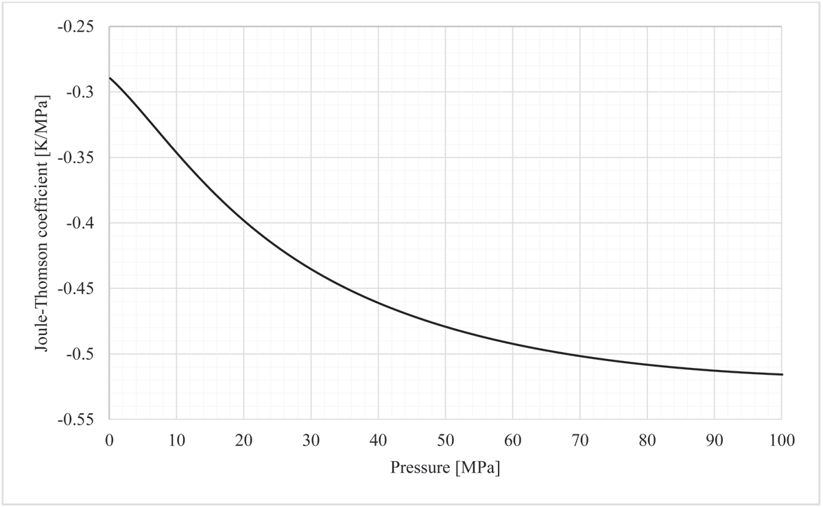
Figure 1
The JT coefficient for hydrogen as a function of pressure at temperature 20°C (Lemmon et al., 2018).
The effect is maximised at the initial stage of refuelling and after the HP tank change, when the pressure in the HP tank may be as large as 90 MPa and onboard storage pressure may be as low as 2 MPa (applicable to the initial stage of refuelling only). Any uncertainty in the prediction of temperature after the PCV might detrimentally impact the efficiency of HRS and refuelling rate, potentially leading to hydrogen temperature and pressure in onboard storage exceeding safety limits specified by regulation (United Nations Economic Commission for Europe, 2023), i.e. 85°C and 1.25 of Nominal Working Pressure (NWP).
The downside of the JT effect on the hydrogen fuelling process was also studied in the work of Johnson et al. (2015) and Wang et al. (2023), where its contribution to temperature increase in onboard tanks was demonstrated. The JT effect also has a role in designing pre-cooling systems. Elgowainy et al. (2017) conducted a techno-economic and thermodynamic analysis of pre-cooling systems and found that the JT effect of the pressure regulator device can significantly increase the temperature upstream of the pre-cooling system which impacts the pre-cooling system design and HRS efficiency. Some experimental tests showed that the temperature at the outlet of the PCV could reach 115°C (Chen et al., 2019). The increased temperature downstream of the regulator valves can affect the material’s robustness within the valve and other HRS and vehicle components. Regulation, codes and standards (RCS) (e.g. ISO standards, 2009; Fuel Cell Standards Committee, 2018, 2020; United Nations Economic Commission for Europe, 2023) define requirements for refuelling protocols. RCS limit the tank’s maximum allowable bulk hydrogen temperature by 85°C so as not to damage the composite and liner of onboard storage tanks during multiple refuelling. Therefore, a CFD model of refuelling must account for the JT phenomenon to correctly simulate the pressure and temperature change at the PCV, and thus its effect on the performance of other equipment of an HRS, to ensure that the supplied to the onboard storage hydrogen temperature and pressure are within the regulated limits.
Some numerical studies have been carried out to model valves. Chen et al. (2019) developed a numerical model to capture the JT effect in a hydrogen pressure regulator in a fuel cell system. Their results showed that although the regulator inlet pressure is an important factor for JT’s temperature increase, the regulator inlet temperature has the most significant influence on its outlet temperature. Rothuizen, Elmegaard and Rokni (2020) developed a mathematical model to study the effect of pressure loss in the piping and other components on the fuelling process. The results showed that the greater the pressure loss in the hydrogen fuelling line, the higher the temperature increase (Rothuizen, Elmegaard and Rokni, 2020). Li et al. (2023) studied the relationships between hydrogen charging parameters and temperature rise due to the JT phenomenon in a valve assembly using analytical analysis. The authors investigated the impact of four different equations of state on hydrogen throttling through a pressure-reducing valve and found that the hydrogen pressure of the high-pressure side of PCV has a greater effect on the temperature difference than the initial hydrogen temperature (Li et al., 2023). This is in contrast to the results of Chen et al. (2019) on the importance of the initial temperature compared to the initial pressure.
On the other hand, although CFD modelling is more computationally expensive, it can provide results with higher accuracy. Turesson (2011) performed a comparison between a 1D hydraulic and a 3D quasi-stationary CFD analysis to model a check valve’s dynamic behaviour. A dynamic mesh technique was used to model the valve in the quasi-stationary CFD model. The geometry changes and mesh updates were done during the simulations to model the valve dynamic behaviour. The results showed that the 1D analysis under-predicts the results and the full 3D dynamic mesh technique is needed to simulate the valve’s transient characteristics. Boqvist (2014) applied the moving mesh technique to model the dynamic closing of a check valve and the results showed that the dynamic mesh was a good way to describe the dynamic behaviour of check valves. Jin et al. (2018) studied hydrogen throttling through a Tesla static pressure-reducing valve using CFD and detailed valve geometry resolution. The effect of valve design parameters, e.g., hydraulic diameter, valve angle, inlet velocity etc., on pressure and temperature at valve outflow was studied, though the valve geometry did not change in the simulations. Kim and Jeong (2021) used the dynamic mesh technique of CFD to investigate the pressure build-up effect on check valve closing characteristics. However, the model was neither validated with experimental data nor was any temperature analysis conducted in their study.
Other studies available in the literature are mainly directed towards optimising a PCV design with limited exploration of the JT effect on the flow passing through the valve. To the authors’ knowledge, there are no publications on CFD models to simulate a realistic PCV performance in a HRS to study the JT effect of hydrogen, which includes the spool motion using the dynamic mesh.
Bourgeois et al. (2018) emphasized the significance of considering the entire refuelling line when studying the filling process. The authors of this study previously developed, validated and published a CFD model to simulate refuelling through the entire equipment of HRS, i.e., the HP and onboard tanks, the PCV, the heat exchanger (HE), valves, piping, etc (Ebne-Abbasi, Makarov and Molkov, 2023; Molkov, Ebne-Abbasi and Makarov, 2023). In these previous studies, the “numerical” PCV was used and the control of mass flow rate was achieved using the “fixed values” technique of ANSYS Fluent (Molkov, Ebne-Abbasi and Makarov, 2023). It was demonstrated that the hydrogen temperature increases while passing through the “numerical” PCV. The temperature augmentation was attributed to the JT effect (Molkov, Ebne-Abbasi and Makarov, 2023). To ensure the accuracy and applicability of the model across various operational conditions at HRS, the pressure reduction at PCV and corresponding temperature increase should be reproduced in simulations with a minimum number of simplifying assumptions. In addition, the integral approach of the “fixed values” method does not allow insights into detailed physical phenomena of heat and mass transfer at the PCV.
The aim of this study is to develop a CFD model of refuelling through the entire equipment of HRS that explicitly incorporates the PCV design with a moving spool using the dynamic mesh technique. This will allow to get insights into the heat and mass transfer at the PCV from the first principles. Dynamic mesh is applied to capture the PCV spool motion regulating the mass flow rate to achieve the required pressure ramp at onboard storage tanks. Properties of hydrogen as real gas are sourced from the National Institute of Standards and Technology (NIST) database (Lemmon et al., 2018). The CFD simulations are compared against the whole 195 s of refuelling in Test No.1 performed by the National Renewable Energy Laboratory (NREL) (Kuroki et al., 2021).
Details of the Validation Experiment
Two tests were performed in the experimental study of the refuelling process carried out at the NREL facility by Kuroki et al. (2021). Test No.1 did not include any leak checks during fuelling, and Test No.2 included two leak checks. Figure 2 depicts the Piping and Instrumentation Diagram (PID) components and locations of pressure and temperature sensors at the NREL experimental facility. The temperature is measured in the HP tanks (TE1, 47 m before the PCV), before and after the PCV (TE2 and TE3, exact distance not available), after the HE (TE4, 2 m after the PCV), and inside two of the onboard tanks (TE5 and TE6) with an accuracy of ±1.5 K. Also, the pressure was measured at the HP tank exit (PT1, 47 m before the PCV), before valve 4 (PT2, 2 m after the PCV), and at the entrance of one of the onboard tanks (PT3, 14.35 m after the PCV) with an accuracy of ±1 MPa (Kuroki et al., 2021). It must be noted that the exact distance of the sensors to the components is not mentioned in the experiment and the mentioned distances are estimated based on the experimental PID diagram.
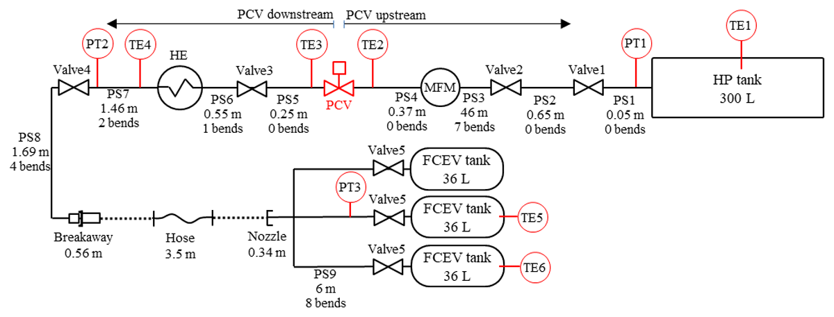
Figure 2
The PID diagram of the NREL experimental HRS.
Test No.1 is selected here for the validation of the CFD model. The initial experimental conditions of Test No.1 are presented in Table 1. The fuelling process is performed using two identical HP tanks in cascade mode. At t = 124 s, when the pressure in the first HP tank drops to approximately 62.5 MPa, the fuelling line is switched from the “depleted” to the second HP tank, which is fully charged, and refuelling continues up to 195 s.
Table 1
Initial experimental conditions of NREL Test No. 1 (Kuroki et al., 2021).
| INITIAL (EXCEPT P TANK) AND AMBIENT TEMPERATURE | HP TANK INITIAL TEMPERATURE | PCV UPSTREAMINITIAL PRESSURE | PCV DOWNSTREAM INITIAL PRESSURE | APRR |
|---|---|---|---|---|
| 296 K | 290.5 K | 88 MPa | 6 MPa | 19.8 MPa/min |
CFD model
Calculation domain
This study focuses on the control of mass flow rate through the PCV using prescribed experimental APRR in onboard storage as an input. The CFD model exploits the benefits of the dynamic mesh technique in the PCV area to simulate spool motion, to get insights into underlying physical phenomena and to compare simulation results against test data and previous simulations using the “fixed values” method (Ebne-Abbasi, Makarov and Molkov, 2023). The internal surfaces of each HRS component are the domain boundaries. The PCV is connected upstream to the 300 L HP tank through 46 m of piping, two valves and a mass flow meter (MFM). The PCV is connected downstream through 15 m of pipes, the HE, two valves, the breakaway, the hose, and the nozzle through a manifold to three equally sized 36 L onboard tanks.
Detailed information on the PCV design is not available in the experimental paper (Kuroki et al., 2021). To model PCV based on a real-life example, the air-actuated hydrogen valve 15V6M071-H2–5MNC (Maximator Gmbh, 2023) is selected in this study to control the pressure ramp in the onboard storage by the spool motion. The reason for selecting this specific valve is that the inlet and outlet diameter, along with the operating pressure limit, are exactly the same as those described in the refuelling experiment (Kuroki et al., 2021). The valve body including wetted parts, i.e., areas where internal surfaces are in direct contact with hydrogen, is made of 316 L (1.4404) stainless steel and the spool is made up of 17-4 PH stainless steel for corrosion resistance (Maximator Gmbh, 2023). Figure 3 (left) shows the cross-section of the actual PCV design. In this study, only wetted parts of the valve were modelled and the body of the PCV along with the actuator section were not included in the calculation domain. The heat transfer through the walls is modelled using the “shell conduction” capability of ANSYS Fluent and will be discussed in the next section. A three-dimensional geometry model was developed for the wetted parts of the PCV and is shown in Figure 3 (right). The spool (orange colour section) can move up and down to control the mass flow rate and provide a target pressure ramp. In the real PCV, the valve spool is supported by both a strong spring and air actuators to limit the lateral displacement and help to actuate the valve. The upward or downward movement of the spool adjusts the flow passing through the PCV (Ye et al., 2022). Except for the diameter of connected pipes, the dimensions of the inner section, including the spool diameter, are not mentioned in the product description. Thus, the PCV flow path dimensions in simulations are estimated using geometrical scaling and sizes shown in Figure 3 (left).
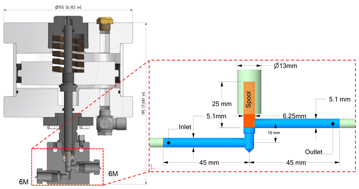
Figure 3
The cross-section of the air-actuated hydrogen valve (Maximator Gmbh, 2023) (left) and the enlarged computational model of the valve’s internal geometry (right).
In this study, the spool movement in the PCV is defined by the requirement to achieve an experimental pressure ramp in the onboard storage. It is realised via an original ad-hoc subroutine code implemented using the User Defined Function (UDF) capability of ANSYS Fluent. For this specific valve, the maximum spool displacement is assumed to be equal to the internal diameter of connected pipes, i.e., 5.1 mm, to exclude an overlap between the spool at the maximum opening and the outlet pipe. Equation (3) is used to specify the relation between the “valve opening”, i.e., displacement expressed in percents, and the spool displacement measured in millimetres (Ye et al., 2022):
where h is the spool displacement distance in mm.
The valve opening area can be calculated as (Pamula and Loo, 2024):
where r is the radius of the outlet pipe in mm.
Figure 4 depicts the relation between the percentage of valve opening versus the percentage of valve opening area.
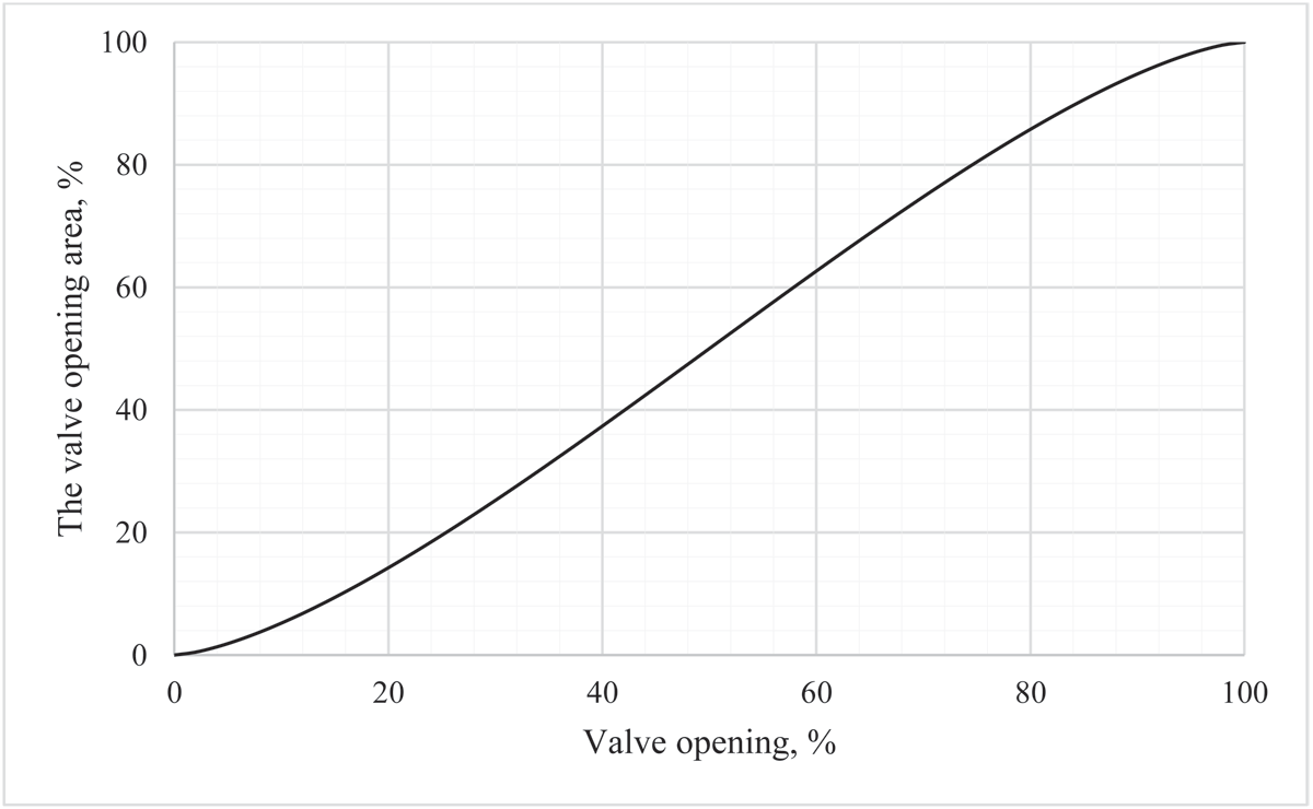
Figure 4
Flow area versus valve opening percentage for the PCV.
Numerical grid and the PCV dynamic mesh details
The numerical mesh is generated using ANSYS Meshing. Tetrahedral control volumes (CVs) were used in the PCV, hexahedral CVs in the rest of the calculation domain and the transition from tetrahedral to hexahedral mesh was realised using pyramid CVs. The entire computational domain (except the PCV) is meshed using 207,252 CVs with a minimum orthogonal quality of 0.7 and an average quality of 0.97. The details for hexahedral mesh are presented in the authors’ previous paper (Molkov, Ebne-Abbasi and Makarov, 2023).
The dynamic mesh technique of ANSYS Fluent is employed to simulate the PCV spool movement and corresponding alterations in the fluid domain mesh over time. Once the domain boundaries are defined and set, the numerical mesh is automatically adjusted during each time step according to the updated positions of these boundaries (Ansys Inc, 2023). In this study, the spool is considered a non-deformable solid body moving along the vertical axis, enabling it to either close or open the valve as needed to provide the required pressure ramp in the onboard storage. The calculation domain deforms in the vertical direction following the movement of the spool. Local re-meshing (Weatherill, 1992) and spring-based smoothing (Batina, 1990) are systematically applied to obtain the grid deformation. The location of the PCV spool changes at each new time step and the mesh is updated accordingly with minimum and maximum CV volume during this process varied between 10–4 mm3 and 3×10⁻³ mm3.
Figure 5 shows the boundary mesh at the initial stage when the valve is closed (Figure 5a) and after deformation when the PCV is 100% open (Figure 5b). Figure 5 presents the same grid comparison but in the central cross-section of the PCV – at the initial stage when the PCV is closed (Figure 5c) and at the moment when the PCV is 100% open (Figure 5d). It must be noted that during deformation, the nodes on the spool mesh are not directly connected to nodes in the fluid zone, as the spool is connected to the fluid through a so-called “interface”. Though the flow path geometry is constantly changing and re-meshed, the spool itself has no deformation or local re-meshing. The PCV is meshed using 37,205 CVs (while it is closed) which could increase to 49,324 CVs when it is 100% open while having a minimum orthogonal quality of 0.8.
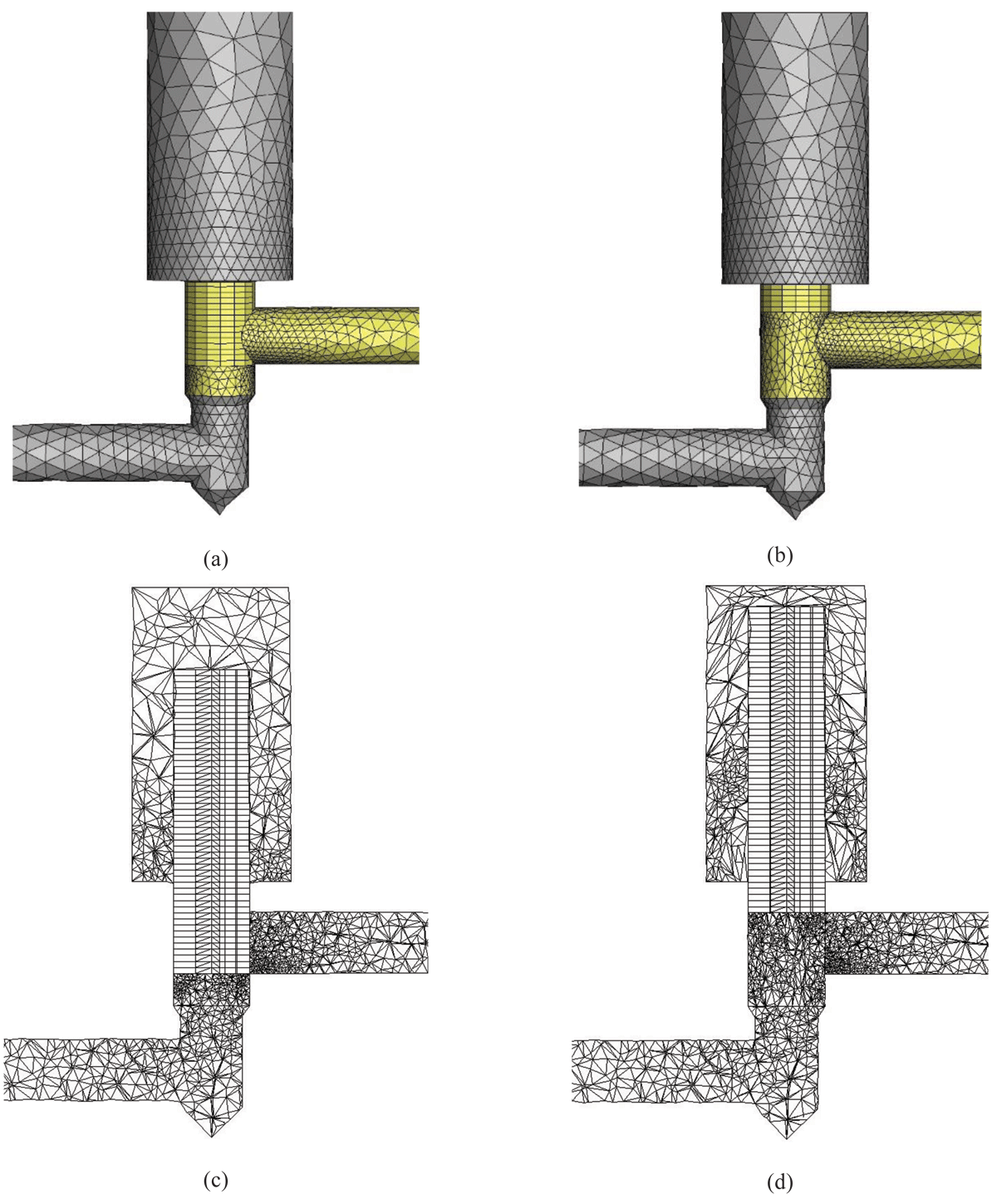
Figure 5
The PCV boundary mesh in the fully closed (a) and fully open (b) states, and the PCV cross-section mesh in the fully closed (c) and fully open (d) states.
Figure 6 shows the calculation domain boundaries along with the PCV domain zoomed in together with locations of the experimental instrumentation: three pressure transducers (PT1-PT3) and six thermocouples (TE1-TE6). TE1 is placed in the centre of the HP tank. The exact distances of the TE2 and TE3 from the PCV, which measures the temperature before and after the PCV, are not specified in the experiment (Kuroki et al., 2021). In the simulation, the temperature “measurements” are done at TE2 and TE3 locations, assuming that they are located at the inlet and outlet of the PCV body respectively, and are on the pipe’s axis at a distance of 45 mm horizontally from the PCV spool axis. The TE4 is placed on the pipe axis, right after the HE, and TE5 and TE6 are placed in the middle of two onboard tanks. The PID components specifications are presented in the Appendix of the paper by Kuroki et al. (2021) and details of their modelling are described in the authors’ previous study (Molkov, Ebne-Abbasi and Makarov, 2023).
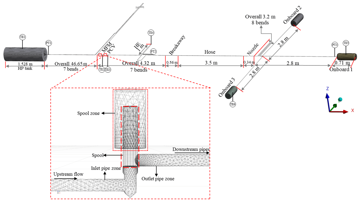
Figure 6
Computational domain comprising the PCV and the other HRS components in the NREL refuelling facility (top), and the three-dimensional zoomed-in area of the PCV with moving spool (bottom).
The motion of the spool is controlled via the UDF and can be based on either a required mass flow rate or a pressure profile, e.g., APRR, in the onboard storage, depending on a refuelling protocol. In this study, the UDF code controls the spool movement to achieve the prescribed APRR using the pressure reading at the pressure transducer PT2 downstream of the PCV (see Figure 6). The block scheme of the UDF code for the PCV spool movement is depicted in Figure 7 and executed in simulations at every time step.
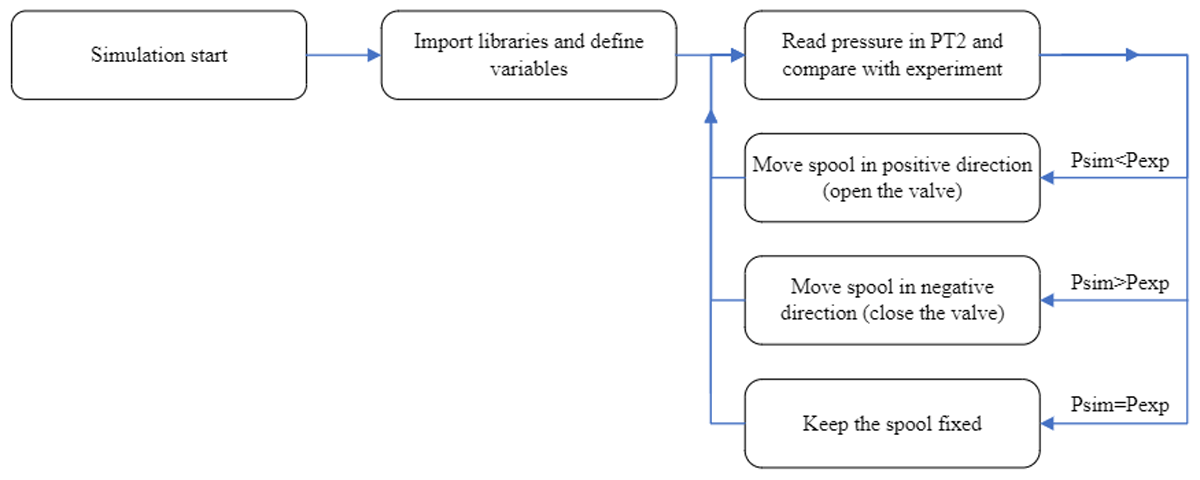
Figure 7
The block scheme of the UDF code to control the spool movement.
The movement of the spool in a positive (opening) or negative (closing) direction is achieved via control of the spool velocity. The velocity of the spool at the current time step, Vi, is assumed to directly depend on the pressure difference between experimental pressure and simulated pressure, and the previous time step velocity, Vi–1:
where the dimensionless pressure difference dpnorms defined as the departure of simulated pressure, psim, from the experimental one, pexp (Molkov, Ebne-Abbasi and Makarov, 2023):
If simulated pressure, psim, is lower than the experimentally measured pressure, pexp, the normalised pressure difference, dpnorm, calculated by Eq. (6), is positive and the UDF increases valve opening speed, Vi, as per Eq. (5) to allow a larger flow rate. Conversely, if the simulated pressure, psim, is larger than the experimental pressure, pexp, the UDF decreases the valve opening speed Vi (potentially down to negative values) simulating the slowdown of the PCV opening. In the case of negative Vi velocity, the spool moves in the opposite direction restricting the flow and decreasing the mass flow rate.
Governing equations and numerical details
Three-dimensional governing equations include unsteady conservation equations for mass, momentum, and energy. Flow turbulence was modelled using the standard k–ɛ turbulence model (Launder and Spalding, 1974) following the findings of Wen et al. (2022) who found that the standard k–ɛ model performs better than the RNG k–ɛ model, realizable k–ɛ model, SST k–ω model and BSL-RSM model in predicting the pressure drop in a check valve using dynamic mesh. On the other hand, Duan et al. (2019) also showed that the standard k–ɛ model performs better than the realizable k–ɛ model for modelling disk valves when , here z is the linear spool displacement and d is the diameter of the inlet pipe. In the current case the condition is satisfied during the most of the refuelling process (see Figure 9 below) and eventually the valve opens up to 71%.
The CFD problem formulation employs the NIST real gas model realised in the form of Thermodynamic and Transport Properties of Refrigerants and Refrigerant Mixtures Database Version 7.0 (REFPROP v7.0) (Lemmon et al., 2018), which provides information on transport and thermodynamic properties (density, enthalpy, entropy, etc.) for different fluids including hydrogen. These property values are called from the NIST database as a function of pressure and temperature in each CV (Ansys Inc, 2023).
The simulations were performed using ANSYS Fluent 2023R1 as the CFD engine (Ansys Inc, 2023). The pressure-based implicit solver was used with the SIMPLE algorithm for pressure-velocity coupling. Convective terms were discretised using a first-order upwind numerical scheme. The simulation of the entire 195 s of the refuelling process with dynamic mesh requires approximately two weeks on a high-performance computing (HPC) cluster equipped with a 128-core CPU and 1 TB of RAM. Though the CFD model was expected to require more RAM space than usual due to dynamic mesh recreation at each time step, the maximum observed peak RAM utilisation during the simulation was approximately 250 GB.
Initial and boundary condition
The initial temperature and pressure in all components, including fluids and adjacent walls, are the same as those outlined in the experimental paper (Kuroki et al., 2021). These parameters were established by the authors in the preceding CFD study (Molkov, Ebne-Abbasi and Makarov, 2023), where control of the mass flow rate was attained via the “fixed values” method. The PCV is assumed to be fully closed at the start of refuelling, while other valves are presumed to be fully open. The walls are characterised as non-slip impermeable surfaces. The ANSYS Fluent “shell conduction” feature is utilised to compute the heat transfer between hydrogen and atmosphere through the component materials. This method calculates conjugate heat transfer across walls in both perpendicular and parallel orientations to the wall axis. Upon specifying material properties such as density, specific heat, thermal conductivity and wall thickness for each segment, the solver automatically generates designated layers of cells, either prismatic or hexahedral shapes, on the wall surface to emulate 3D heat conduction [31]. This modelling approach accounts for the prescribed wall thicknesses, pertinent thermal properties of materials and convective heat transfer on the external surface of the wall. The heat transfer coefficient for heat exchange between the outer pipe surface and ambient atmosphere is set at 7 W/m2/K, aligning with the conclusions of the study of Simonovski et al. (2015). As the thermal mass of the valves is not available in the experiment (Kuroki et al., 2021), it is assumed that valves have the same external diameters and materials as their upstream pipes.
The parameters of the HE are not provided in the experimental paper [28]. The HE modelling followed the same technique as in the numerical study (Molkov, Ebne-Abbasi and Makarov, 2023): the HE is presented in the calculation domain design as a pipe with a length of one meter, and the equivalent HE piping diameter is estimated based on the flow coefficients provided in the experiment reference (Kuroki et al., 2021). The “fixed values” feature of ANSYS Fluent was employed to ensure that the hydrogen temperature at the HE outflow remained consistent with that of the experiment. The latter was achieved using a UDF as well.
The transition from the first “depleted” HP tank to the second one with higher pressure is modelled by overwriting (patching) the simulated hydrogen pressure and temperature in the numerical HP tank and its shell layer model at t = 124 s with the initial values corresponding to temperature and pressure as in the first HP tank.
Results and Discussion
This section outlines the comparison of simulations against experimental data in Test No.1 as conducted by Kuroki et al. (Kuroki et al., 2021). Since the original experimental transients were not available to the authors, the figures presented in the experimental paper (Kuroki et al., 2021) were digitised to validate the simulations.
Accuracy of the experimental data input (APRR and the HE temperature)
The experimental APRR and the HE outflow temperature serve as input parameters. The CFD model accuracy will rely on how closely the PCV spool displacement and the cooling of hydrogen within the HE, both controlled using UDF, reproduce the experimentally measured pressure after the PCV and the experimentally measured temperature after the HE. The inputs of the UDF consist of (a) the experimental pressure at the PT2 sensor location, located 2.5 m downstream of the PCV, expected to yield APRR = 19.8 MPa/min, and (b) the digitised experimental temperature at the TE4 placed just after the HE. The exact distance between TE4 and the HE in the experiment is not specified. In the simulations, it is assumed that the TE4 is positioned at the interface of the HE and its downstream pipe. The locations of the sensors are illustrated in Figures 2 and 6.
The experimental pressure is approximated using a polynomial function:
where t is time (s).
Similarly, the experimental temperature in the TE4 location is approximated using Eq. (8) and Eq. (9):
The UDF realises presented in Figure 7 implements an algorithm to control the movement of the PCV spool, continuously monitoring downstream pressure and initiating the valve to open and close as necessary to achieve the prescribed pressure ramp rate. Figure 8 (left) depicts the comparison of experimental and simulated pressure at sensor PT2. The UDF successfully reproduces the pressure within a 3% deviation from the experimental value and less than 1% error compared to its input approximation of Eq. 7. The simulated pressure transient appears smoother compared to the experimental one, likely due to the non-inertial behaviour of the numerical PCV’s spool in the simulations.
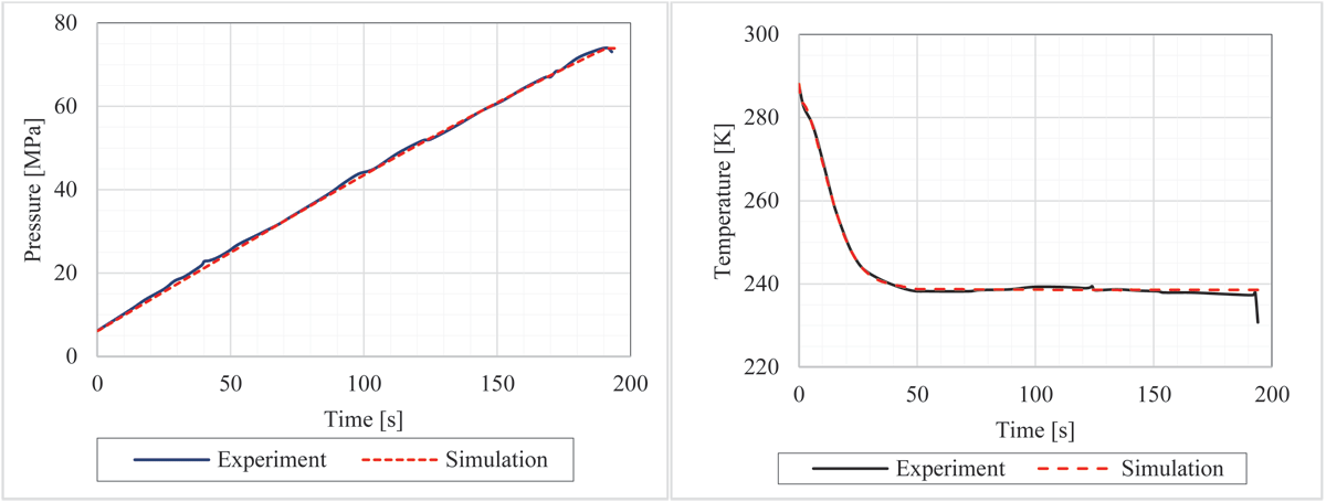
Figure 8
Pressure in PT2 located 2.5 m after the PCV (left); hydrogen temperature at the HE exit (right).
Figure 8 (right) presents the comparison of experimental and simulated temperature at the sensor TE4 location just after the HE exit. The simulated HE outflow temperature closely matches the experimental data with a maximum deviation of 3.5% compared to the experiment and less than 1% deviation compared to the input correlations of Eq. (8) and (9).
The authors conclude that the procedure for controlling the PCV spool motion and the HE temperature is sufficiently accurate for automatic simulation of the PCV and the HE functions, ensuring that the APRR and temperature align with the data recorded in the experiment, as presented in this paper, or as prescribed by a fuelling protocol for arbitrary HRS conditions.
The PCV spool displacement and mass flow rate
The accurate attainment of the pressure ramp rate in onboard storage relies on achieving the correct mass flow rate accounting for the continuous changes in temperature and pressure across the entire set of HRS components. Figure 9 compares experimentally measured and simulated mass flow rates along with the PCV spool displacement. The visual disparity observed between the measured (oscillating) and simulated (smooth) mass flow rates could be explained by several factors. Firstly, the experimental mass flow rate was derived from the measurement of the HP tank weight, which could introduce oscillations due to recoil force. Secondly, the inertia of the real PCV spool movement mechanism may differ compared to the non-inertial “numerical spool” used in the simulations. These differences may describe the discrepancy between the oscillatory nature of the experimental mass flow rate and the smoother (non-inertial) simulated mass flow rate.
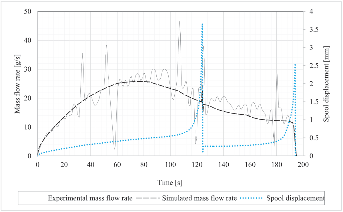
Figure 9
Experimentally measured and simulated mass flow rate along with the PCV spool displacement.
Figure 10 demonstrates that although the allowable axial movement of the PCV spool is limited to 5.1 mm, the maximum simulated spool displacement reaches 3.63 mm, resulting in 71% of the PCV possible spool travel distance. This is equivalent to 75% of the PCV opening area. At the beginning of the refuelling process, when the spool of the PCV begins to move, the mass flow rate initiates from an initial zero value. The maximum simulated mass flow rate is achieved at t = 80 s after the start of refuelling. Subsequently, despite a further increase in the spool displacement, the mass flow rate decreases due to a pressure drop in the HP tank upstream of the PCV. The spool movement control procedure, defined by Eq. 5 and Eq. 6, continues to regulate the simulated pressure towards the experimental value (Figure 8, left) by increasing the spool displacement velocity, as evidenced by the rising slope of the spool displacement (dotted line in Figure 9).
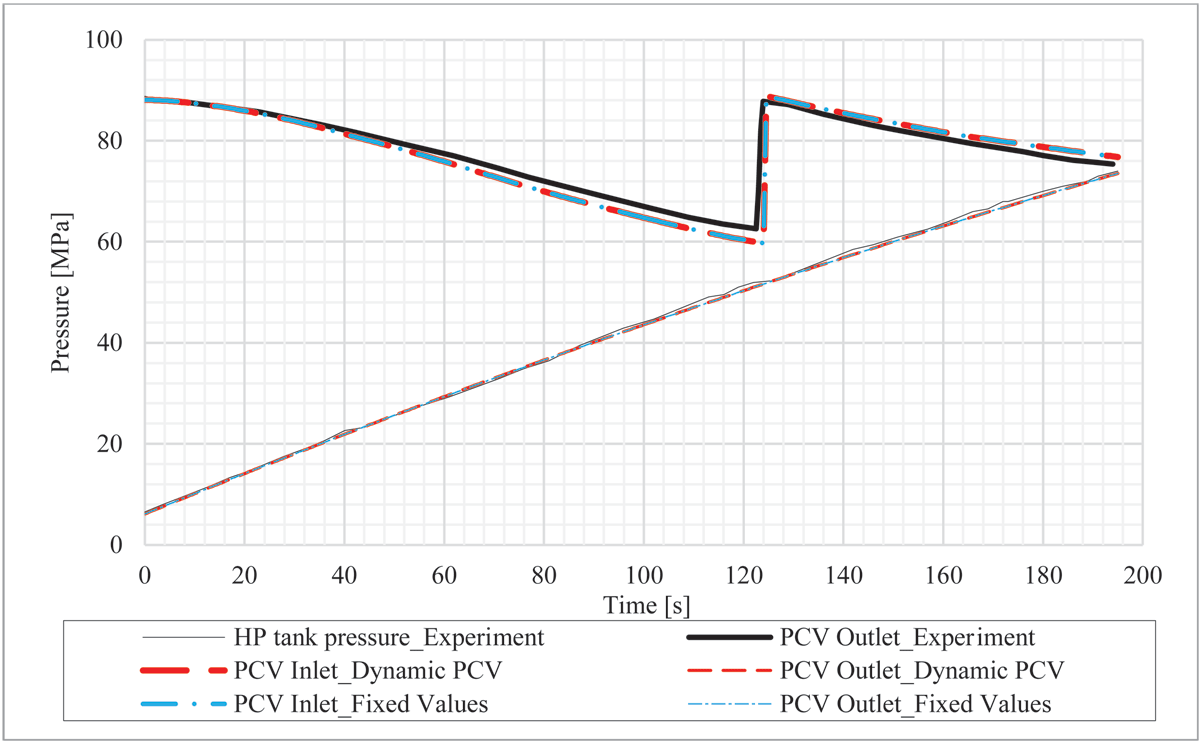
Figure 10
Experimental and simulated (dynamic mesh and fixed values methods) pressure dynamics upstream and downstream of the PCV. Note: experimental pressure upstream is measured at the HP tank exit (47 m from the PCV).
The sudden drop in the spool displacement graph observed in Figure 9 at t = 124 s is attributed to the replacement of the “depleted” HP tank with a second tank possessing a higher pressure of 88 MPa at that moment. The abrupt change to higher pressure in the fuelling line upstream of the PCV necessitates maintaining the pressure at PT2 at the same level, thus resulting in a decrease in the spool displacement down to 0.28 mm.
Subsequently, during the refuelling from the second HP tank, i.e., t = 124–195 s, the spool behaviour mirrors that observed during the refuelling from the first HP tank, i.e., t = 0–124 s. Specifically, the PCV spool velocity gradually increases to counteract the HP tank’s decreasing pressure and to ensure that the simulated pressure dynamics at the PT2 location follow the prescribed APRR as defined by Eq. 7. At t = 195 s, the fuelling process terminates, leading to a decrease in the spool displacement to zero, signifying the closure of the PCV.
Pressure and temperature before and after PCV
The experimental and simulated pressure at the inlet and outlet of the PCV is illustrated in Figure 10. Additionally, the results from the previous study (Ebne-Abbasi, Makarov and Molkov, 2023), where the flow was regulated using the “fixed values” method, are also included for comparison. It is worth noting that the experimentalists did not measure pressure upstream of the PCV but rather in the HP tanks, which are situated approximately 47 m away from the PCV. However, in the simulation, pressure is measured at the inlet and outlet of the PCV body, located 45 mm horizontally from the PCV spool axis. This is a likely reason why the experimental pressure in Figure 10 appears somewhat higher than the simulated pressures recorded in simulations just upstream of the PCV inlet. This difference, i.e. pressure drop from the HP tank to the PCV, increases gradually and reaches about 4 MPa just before the first HP tank changes to the second one. Figure 10 also displays the experimental HP tank pressure. The key finding is that both methods, i.e., the dynamic mesh PCV and the fixed values, simulate the same pressure upstream and downstream of the PCV. While the fixed values method simulates faster, it cannot get insights into details of underlying physical phenomena inside the PCV. At the end of refuelling, the pressure difference upstream and downstream of the PCV decreases, and at t = 195 s, the PCV closes to terminate the refuelling process once the target pressure in onboard storage is reached.
The experiments (PRHYDE – Deliverable 6.7, 2022) demonstrated that the flow coefficient directly impacts the pressure drop, which in turn influences the temperature in the compressed hydrogen storage system (CHSS). The larger the throttling effect is, the stronger is expected to be the Joule-Thomson heating. Figure 11 illustrates both the experimental (solid black lines) and the simulated (red dashed lines) temperatures at identical locations, specifically at the inlet and outlet of the PCV where TE2 and TE3 sensors are positioned.
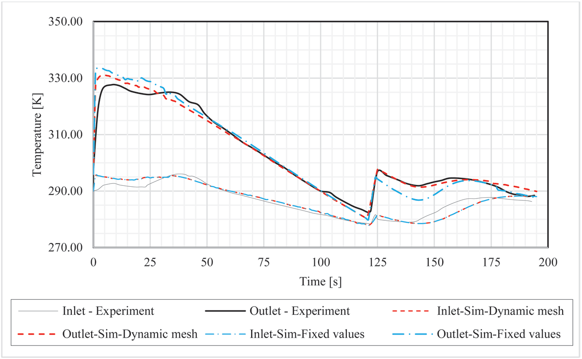
Figure 11
Experimental and simulated (dynamic mesh and fixed values methods) temperature dynamics at the inlet (TE2) and outlet (TE3) of the PCV.
The highest pressure difference across the PCV is at the start of refuelling. This corresponds to the largest increase in temperature by 40 K due to the JT effect during throttling at the PCV. As refuelling progresses, the pressure drop at the PCV gradually decreases. By t = 124 s, before the HP tank replacement, the pressure difference across the PCV decreases to 8 MPa. Consequently, the increase of temperature at the PCV diminishes to 5 K in the test and 3.5 K in the simulations.
The replacement of the HP tank causes a pressure jump upstream of the PCV, resulting in an increase of pressure difference across the PCV from 8 MPa to above 36 MPa (refer to Figure 10). This surge is associated with a notable increase in temperature due to the JT effect: from 3.5 K before switching to the second HP tank to 15.5 K when refuelling starts again from the fully charged second HP tank. At the end of refuelling the pressure drop decreases again, this time to 4 MPa, and the temperature rise due to the JT effect and associated heat transfer between hydrogen and HRS equipment reduces to about 2 K.
According to Figure 11, the simulated temperature dynamics closely follow the experimental transients and the model accurately simulates the pressure gradient and temperature increase in the fuelling line due to the JT effect. The CFD model with dynamic mesh provides a better agreement between experimental and simulated temperatures at the PCV outflow compared to the “fixed values” method [16]. The larger difference observed between simulated and experimental temperatures at outflow for the “fixed values” simulations may be attributed to the inadequate consideration of the PCV thermal mass (not described in [32]), whereas the present CFD model explicitly captures the major features of the PCV design with corresponding material properties.
It must be noted that the exact locations of temperature sensors TE2 and TE3 close to the PCV were not reported in the experimental paper. As mentioned earlier, the simulation temperature is recorded at the inlet and outlet of the PCV body, where the “simulated” TE2 and TE3 sensors are located 45 mm horizontally from the PCV spool axis on the pipe’s centreline. Figure 12 displays the temperature and velocity at the cross-section of the pipe at the PCV inlet (TE2 location) and outlet (TE3 location) to show the extent of the uniformity of velocity and temperature at the TE2 and TE3 locations. Figure 12 (top, right) and Figure 12 (bottom, right) illustrate the velocity and temperature profiles across the pipe cross-section at the TE2 and TE3 locations respectively. Remarkably, the velocity reaches its peak of 9 m/s at the pipe’s centre and gradually decreases to zero at the walls due to the no-slip boundary condition. Simultaneously, the temperature peaks at 295.700 K along the walls, gradually decreasing to 295.695 K at the centre, i.e. the temperature is practically uniform. The flow velocity and kinetic energy are maximised at the pipe axis. On the other hand, the velocity and temperature changes in their relevant profiles on the PCV exit (TE3) are more noticeable. Figure 12 (right) depicts the velocity and temperature profiles along the centreline of the cross-section of the pipe at the TE3 location. Notably, the velocity attains its apex of 68 m/s at the pipe’s centre and gradually diminishes to zero at the walls due to the no-slip boundary condition. Concurrently, the temperature peaks at 330.5 K along the walls, gradually tapering to 329.5 K at the centre, where the flow velocity and kinetic energy are maximised.
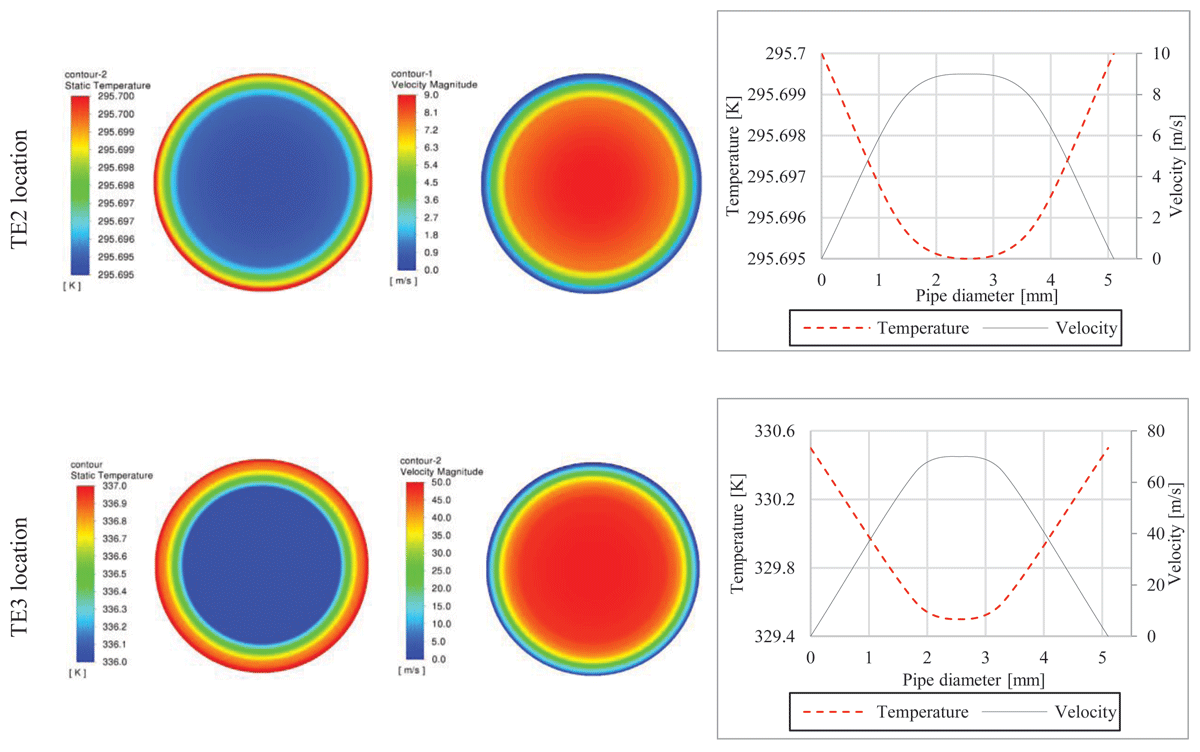
Figure 12
Temperature (top, left), velocity distribution (top, centre) across the pipe cross-section, temperature and velocity profiles across the pipe cross-section at the PCV inlet (TE2 location) (top, right); temperature (bottom, left), velocity distribution (bottom, centre) across the pipe cross-section, and temperature and velocity profiles across the pipe cross-section at the PCV outlet (TE3 location) (bottom, right).
From a thermodynamical standpoint, Figure 13 provides insights into the temperature increase after the PCV due to the JT effect. The figure illustrates the isenthalpic curves of hydrogen spanning a broad range of temperatures and pressures. These curves are derived by processing data from the NIST database (Lemmon et al., 2018). At any given point along the curve, the slope represents the JT coefficient value. The location of points where the JT coefficient equals zero is termed the inversion curve (Molkov, 2012).
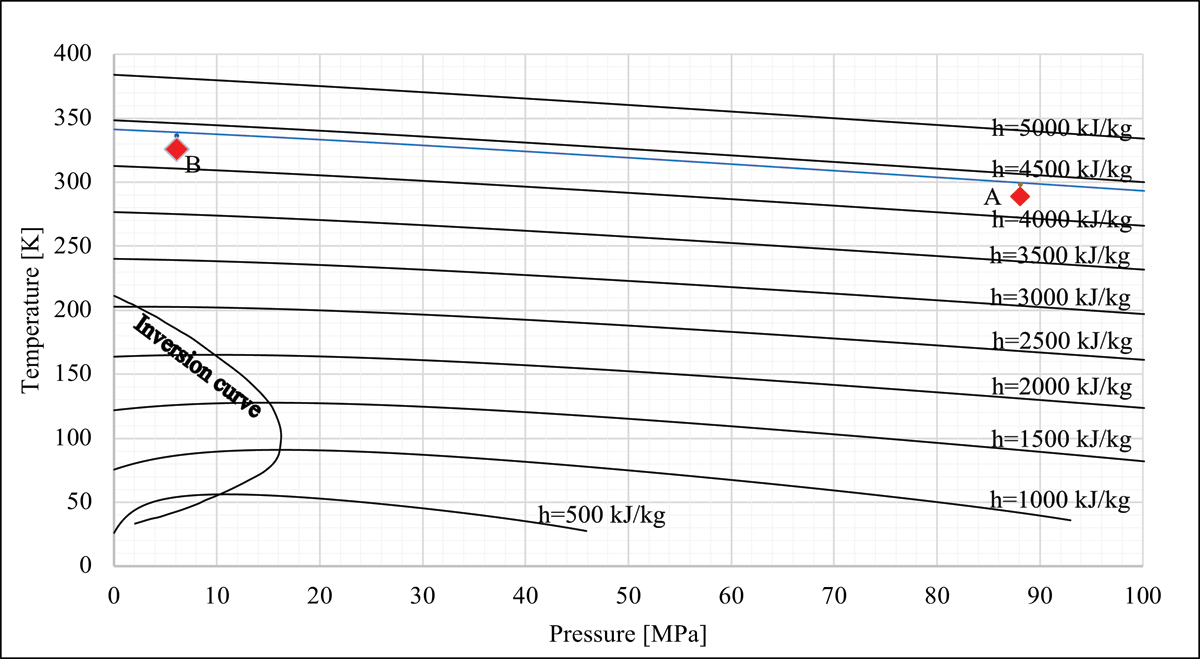
Figure 13
Isenthalpic curves (solid lines) with their corresponding enthalpies (h) and inversion curve (dashed line) for hydrogen.
In the idealised scenario, as the flow passes through a throttling valve, there is neither sufficient time nor a large enough area for any effective heat transfer to occur. Therefore, the flow can be assumed to be adiabatic, as stated in Cengel (2004). Moreover, as the enthalpy of the flow at the inlet and exit of a throttling valve are the same, the process of throttling through a valve is sometimes referred to as isenthalpic (Cengel, 2004). While real-world factors such as irreversibility, non-ideal gas behaviour and heat exchange with the surroundings prevent the process from isenthalpic behaviour, Figure 13 serves as a valuable starting point to predict the results.
For demonstration purposes, let’s consider the pressure and temperature change at t = 6 s when the experimental temperature experiences a significant increase due to the JT effect, while the pressure and temperature values are not changing violently compared to the start of the refuelling process. Assuming an isenthalpic and adiabatic throttling process with no heat transfer and negligible friction losses, where the PCV inlet pressure is 88 MPa and the temperature is 296 K (represented as thermodynamic state “A” in Figure 13), with the total enthalpy of 4456.9 kJ/kg according to the NIST database (Lemmon et al., 2018). Moving along the isenthalpic curve toward the outlet pressure of 6 MPa, theoretically, we should reach a temperature of 330.5 K (depicted as thermodynamic state “B” in Figure 13). However, the experimentally recorded temperature is 327.7 K, and the simulated temperature is 329.5 K, i.e. slightly below the theoretical value for the adiabatic process. This discrepancy can be attributed to the presence of heat losses (non-adiabaticity of the real and simulated processes) from heated hydrogen to the equipment, as well as the presence of wall and viscous frictions in both the experiment and the simulations.
Notably, the temperature in the simulation, 329.5 K, is higher than the experimental value, 327.7 K. The discrepancy may arise from disparities between the actual and simulated models of the PCV, resulting in varied thermal mass, etc. The discrepancy can be associated also with the unspecified sensor location in the experiment, thereby emphasising the significance of knowing the precise sensor position to achieve congruence between the simulations and the experiment.
Figure 11 also reveals a similar yet slightly lower accuracy in simulated temperature dynamics compared to the findings of the previous study [16], where the PCV was treated as a simple pipe and the flow was controlled using the “fixed values” technique (depicted by blue dash-dotted lines). The figure suggests that the explicit PCV resolution accounting for its actual design results in better agreement with the experimental temperature after the PCV. Nevertheless, the “fixed values” method still yields acceptable results while significantly reducing the simulation time by an order of magnitude (two days compared to two weeks for dynamic mesh). The maximum departure from the experimentally recorded temperature for the dynamic mesh model is 3 K, representing 1% of the maximum temperature rise due to the JT effect in the considered experiment. In contrast, the deviation for the “fixed values” method was 5 K, representing 1.5% of the maximum temperature rise. This finding highlights the importance of considering trade-offs between simulation accuracy and computational resources when selecting simulation methods for complex systems like the one in the current study.
Figure 14 shows the positions of the temperature recordings in simulations TE2 and TE3 (both 45 mm from the PCV spool axis at the centreline of the pipes). It also illustrates the temperature contour in the PCV cross-section at the same time of 6 s when the temperature increases after the PCV is still high, while not fluctuating dramatically. Notably, the temperature at the location of the downstream sensor TE3 is increased. However, closer to the gap between the PCV body and the spool, the temperature significantly decreases from 296 K before the PCV to 196 K in the “blue colour” zone. This observation can be elucidated by analysing the velocity contour.
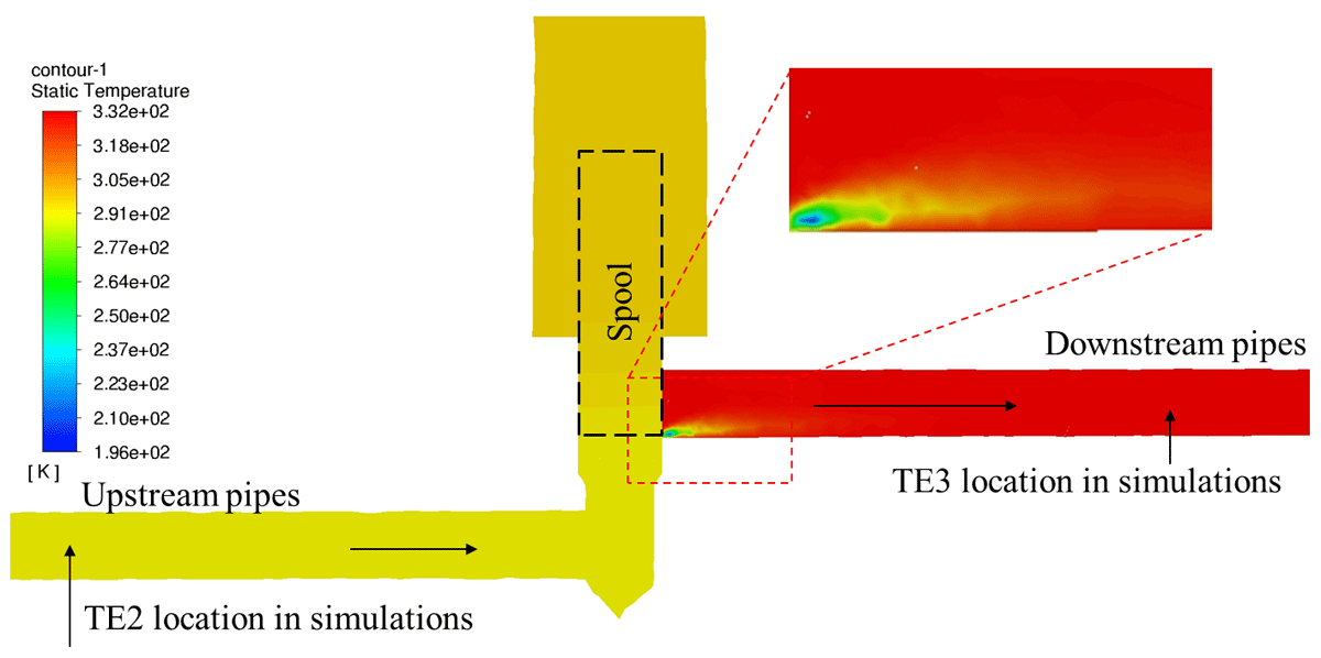
Figure 14
Hydrogen temperature in the PCV cross-section at the initial stage of the fuelling process at t = 6 s.
Figure 15 shows the pressure distribution (top, left) and velocity distribution (top, right) in the cross-section of the PCV. Examination of the velocity contour in the PCV cross-section, as presented in Figure 15 (top, right), reveals that the hydrogen flow near the opening can attain supersonic velocities, reaching up to 1956 m/s, characteristic of hydrogen supersonic flows. The speed of sound in hydrogen at 196 K is 1068 m/s.
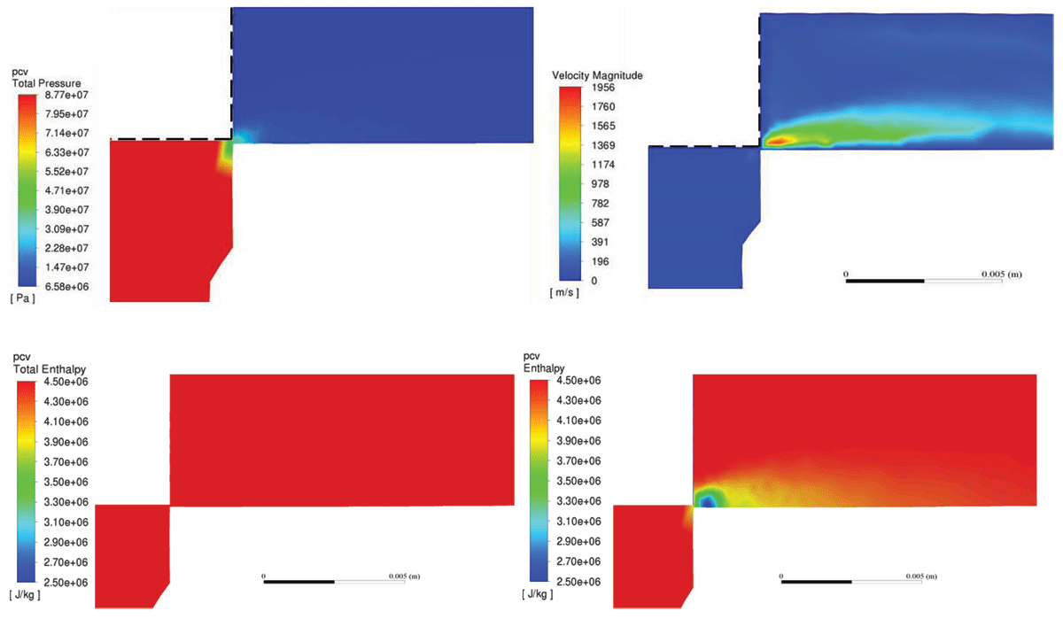
Figure 15
Pressure distribution (top, left), velocity field (top, right), total enthalpy H (bottom, left) and enthalpy h (bottom, right) distribution in the PCV cross-section at t = 6 s.
Comparing the velocity contour (Figure 15, right) with the temperature contour (Figure 14) shows that the temperature of the gas decreases in areas where velocity is very high. This phenomenon can be explained by analysis of the total energy equation:
where E is total energy, u is internal energy, v is velocity, h is enthalpy, p is pressure and ρ is density.
Assuming no friction or heat loss, the principle of conservation of the total energy dictates that the total energy of the gas remains constant after expansion. As the gas expands, internal energy is converted into kinetic energy, resulting in a temperature decrease. This is observed in areas with high velocities, specifically near the PCV opening where gas experiences rapid expansion and acceleration. Conversely, as hydrogen moves away from the PCV spool, it decelerates, converting kinetic energy back to internal energy. Consequently, the temperature rises, as depicted in Figure 14. This causes a continuous competition between the effect of adiabatic expansion, which tends to decrease temperature due to the conversion between internal and kinetic energies as flow accelerates, and the JT effect which tends to increase temperature. This interplay between velocity and temperature highlights the important relationship between fluid dynamics and thermodynamics governing gas flow within the PCV.
Figure 15 also compares the enthalpy h (bottom, right) with the total enthalpy, bottom, left). The enthalpy decreases in areas where kinetic energy increases (indicated by blue-coloured areas) and increases again when flow decelerates. Analysis of total enthalpy reveals that total enthalpy in the PCV upstream and downstream (assessed in TE2 and TE3 locations) only differs by –0.5% (Figure 15, left). This slight difference can be explained by the energy conservation equation (Landau and Lifshitz, 1987):
where u internal energy, v is velocity vector, v is velocity magnitude, σ is the stress tensor term, κ is thermal conductivity and T is temperature. The expression on the left-hand side denotes the rate of change of energy per unit volume of the fluid. On the right side, the first term represents the flux of energy due to mass transfer, the second term represents the flux of energy due to friction, and the last represents the flux of energy due to thermal conduction (Landau and Lifshitz, 1987).
As per Landau and Lifshitz (1987), the left term is called “the rate of change of total energy”, whereas the combination of terms on the right is referred to as the “flux of energy”. Under assumptions of steady-state flow, adiabatic boundaries, no work performed on the system, no friction, and negligible heat transfer within the fluid, the equation olds. This implies that the enthalpy inflow upstream of the PCV and the enthalpy outflow downstream of the PCV should be equal. That is the reason throttling valves are sometimes referred to as isenthalpic devices (Cengel, 2004).
To evaluate the effect of wall friction and heat transfer on the change of energy of the system, two additional simulations were performed: one with no heat transfer (isolated wall boundaries) and the other one without friction (slip condition) and no heat transfer (heat transfer coefficient of zero). Table 2 compares the total enthalpy at the inlet (TE2 location) and outlet (TE3 location) of the PCV for these scenarios. In the scenario where neither heat transfer nor friction is present, the total enthalpy change is only –0.033%. It is assumed that this difference is primarily attributed to the internal friction in the gas. For the scenario with non-slip walls, the difference is –0.038%, a value closely resembling the previous case. This observation suggests that wall friction within the valve does not play a major role in affecting the energy flux. Conversely, the inclusion of heat transfer in the simulation results in a total enthalpy change of –0.525%. Therefore, heat transfer emerges as the main reason for the loss of energy flux in the PCV.
Table 2
Comparison of total enthalpy at t = 6 seconds at the inlet and outlet of PCV (TE2 and TE3 location).
| CASE | TOTAL ENTHALPY AT THE INLET (TE2) [J/kg] | TOTAL ENTHALPY AT THE OUTLET (TE3) [J/kg] | DIFFERENCE (%) | TEMPERATURE AT TE3 [K] |
|---|---|---|---|---|
| Ideal case, Isenthalpic expansion (using NIST data) | 4,473,342 | 4,473,342 | 0% | 330.5 |
| Slip wall conditions, No heat transfer | 4,473,342 | 4,471,888 | –0.033% | 330.9 |
| Non-slip conditions, No heat transfer | 4,473,342 | 4,471,654 | –0.038% | 331.1 |
| Non-slip conditions, With heat transfer | 4,473,342 | 4,449,820 | –0.525% | 329.5 |
Comparing the temperature at the TE3 location, it turns out that the temperature in scenarios with no heat transfer is higher, even when compared to the NIST isenthalpic expansion condition where the temperature reaches 330.5 K. This can be attributed to either the fact that temperature taken in TE3 location on the pipe axis is different from the averaged through cross-section area temperature or losses incurred due to wall and viscous friction. These losses cause the system’s kinetic energy to transform into thermal energy due to the resistance encountered. As anticipated, the scenario with heat transfer exhibits the lowest temperature at the PCV outlet (TE3 location). This comparison emphasizes the dynamic relationship between kinetic energy, friction and viscous losses, and enthalpy within the PCV assembly and their collective influence on the thermodynamic parameters of the refuelling system.
Impact of the JT coefficient: “numerical refuelling” with methane and air
To assess the effect of the JT coefficient value, the developed CFD model with detailed PCV resolution and dynamic mesh, was applied to simulate the imaginary “refuelling” of methane and then air as they have positive JT coefficients contrary to hydrogen. The simulations were performed for the same equipment of HRS to see the difference with hydrogen refuelling. Figure 16 depicts that despite having the same inlet temperature for all simulations, the PCV outlet temperature is different. The PCV outlet temperature increases for hydrogen, while it decreases for air and methane.
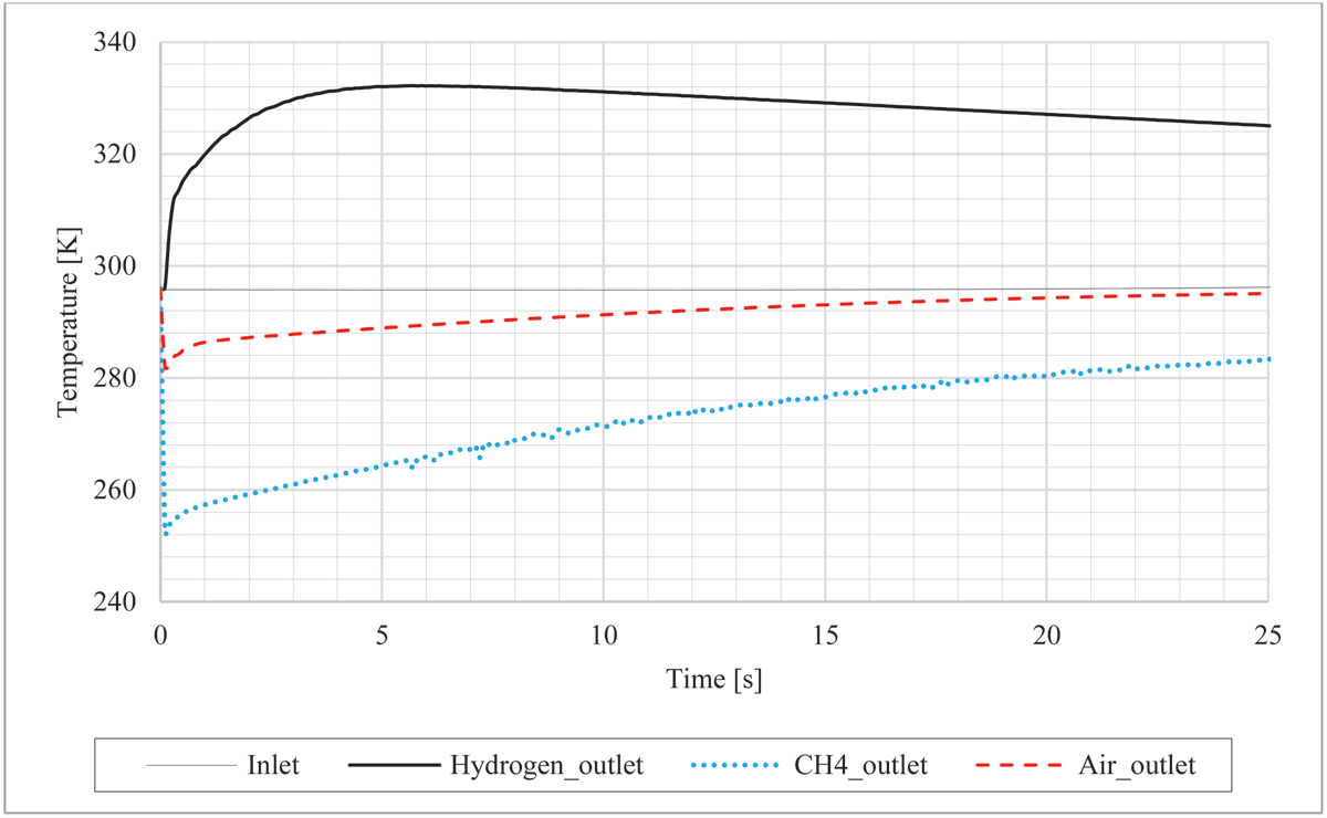
Figure 16
The joint effect of the heat transfer and the JT phenomenon on the PCV outlet temperature for the same HRS and initial conditions for three gases: hydrogen, air and methane.
Figure 16 compares temperatures at the PCV inlet and outlet obtained in the CFD simulations for hydrogen, air and methane during the initial 25 s of the gas transfer process. At t = 1 s, for the same inlet PCV temperature of 296 K, the PCV outlet temperatures for air decreased to 282 K (a reduction of –14 K) (isenthalpic expansion using the NIST database gives 281.6 K (Lemmon et al., 2018)). For methane, the outlet temperature decreases to 251 K, i.e. by –45 K (isenthalpic expansion value using the NIST database is 247.2 K). However, the situation for hydrogen is reversed due to its negative JT coefficient. For hydrogen, the PCV outlet temperature increases to 321 K, i.e. by +25 K, with further increases to 329.5 K at t = 6 s (isenthalpic expansion using the NIST database gives 330.5 K). The outlet temperature values obtained by the CFD model are above the NIST values for air and methane and below the NIST values for hydrogen. This is in line with the physics of the process indicating that heat transfer is directed in the CFD simulations from HRS equipment to gas (air and methane) and in the opposite direction from gas to the equipment for hydrogen. It is worth mentioning that over time, the temperature of cooled gases after the PCV (air and methane) gradually increases after the initial drop, and heated gas (hydrogen) slowly decreases after the initial larger increase. This underlines the complex process of heat and mass transfer for gases with different and continuously changing JT coefficients.
Temperature and pressure at onboard tanks
Figure 17 shows the comparison between experimental and simulated pressures (left) and temperatures (right) in the onboard tanks. The CFD model effectively reproduces the temperature trend in the onboard tanks during the entire fuelling process with a deviation of less than 5 K and the final temperatures exhibiting a deviation of only 3 K. This deviation is comparable to the experimental temperature oscillations in onboard Tank 2 during refuelling. The deviation of simulated pressure from the experimental one is less than 0.95 MPa which is ±1.5% across the entire duration of the refuelling process. Notably, this deviation is within the pressure transducer accuracy of ±1.0 MPa.
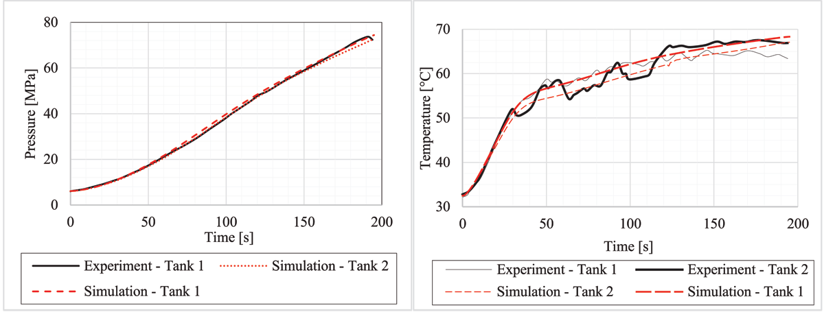
Figure 17
Experimental and simulated temperatures (left) and pressures (right) in two of three onboard tanks.
Conclusions
The originality of this work is in the development of the CFD model with an explicit numerical resolution of the PCV with spool displacement to regulate the required pressure ramp after the PCV in a hydrogen refuelling station. Employing the dynamic mesh technique to simulate PCV spool movement allows to avoid modelling assumptions and simplifications that might compromise the accuracy of refuelling simulation. This approach provided valuable insights into the underlying physical phenomena of heat and mass transfer at the PCV, including the JT phenomenon. The PCV geometry was modelled based on a real valve design, ensuring practical relevance. The PCV spool motion was controlled by an original algorithm grounded in the sampling of numerical pressure deviation from the experimental pressure, as defined by the prescribed APRR for NREL Test No.1. The algorithm was implemented using a user-defined function of ANSYS Fluent. The results revealed that during the throttling process, the total enthalpy of gas decreased by 0.525%. Consequently, for future engineering applications such as valve and/or PCV performance analysis, designing HRS components, and developing numerical models, the assumption of an isenthalpic process for high-pressure hydrogen flow in valves remains valid.
The significance of this study lies in developing and validating a CFD model, which serves as a contemporary engineering tool for the design of HRS equipment and fuelling protocols. This model incorporates the Joule-Thomson effect and considers heat and mass transfer at the PCV, impacting pressure and temperature dynamics at various locations of HRS. It enables the design of innovative HRS components and refuelling protocols based on pressure ramps in onboard storage or mass flow rate.
The rigour of this work is in the validation of the model against the available hydrogen refuelling data generated by NREL. The validation process encompasses a comprehensive examination of temperature and pressure measurements taken upstream and downstream of the PCV as well as pressure and temperature profiles throughout the individual components of a hydrogen refuelling station, including onboard tanks, PCV, HE and HP tanks.
Funding Information
This research has received funding from the Engineering and Physical Sciences Research Council (EPSRC) of the UK through: the Centre for Doctoral Training in Sustainable Hydrogen (“SusHy”), Grant number EP/S023909/1; UK National Clean Maritime Research Hub (UK-MaRes Hub), Grant number EP/Y024605/1; Tier 2 Northern Ireland High-Performance Computing facility (NI-HPC “Kelvin-2”), Grant number EP/T022175/1. Funding was also received from Fuel Cells and Hydrogen 2 Joint Undertaking (now Clean Hydrogen Partnership) under the European Union’s Horizon 2020 research and innovation programme through the SH2 APED project under Grant Agreement No. 101007182. Funded by the European Union. Views and opinions expressed are however those of the author(s) only and do not necessarily reflect those of the European Union or the Clean Hydrogen Partnership. Neither the European Union nor the Clean Hydrogen Partnership can be held responsible for them.
Competing Interests
The authors have no competing interests to declare.