
1 Introduction
Computational models of music perception and cognition require tools for quantifying the similarity of pitch collections, the consonance of chords, and the structural properties of scales and rhythms. Over the past 15 years, a body of such tools has been developed around the expectation tensor framework introduced in Milne et al. (2011), together with complementary Fourier‑based distributional measures (Milne et al., 2017), sensory roughness models (Sethares, 1993), and a suite of structural features for scales and rhythms (Milne et al., 2023a).
The expectation tensor framework—in which weighted multisets of pitches or time points are embedded into continuous probability‑like densities, smoothed by a Gaussian kernel that models perceptual uncertainty—provides a unified foundation for measuring both the similarity of two pitch or time‑point collections (via the cosine similarity of their densities) and the structural complexity of a single collection (via the entropy of its density). Crucially, with the exception of spectral enrichment (which is specific to pitched sounds), the underlying mathematics of all these measures is domain‑agnostic: the same framework applies to pitch and rhythm, with only the interpretation of the domain changing: pitches on a pitch line or pitch‑class circle, or onsets on a timeline or time‑class circle.
These measures have been applied across a wide range of music cognition contexts. Spectral pitch class similarity (SPCS)—the cosine similarity of spectrally enriched, octave‑periodic monad densities—has been validated as a predictor of probe tone ratings and tonal hierarchies (Milne et al., 2015), perceived tonal affinity with microtonal melodies and inharmonic spectra (Milne et al., 2016), perceived triadic distance (Milne and Holland, 2016), individual differences in harmony perception (Eitel et al., 2024), and contextual tonal stability in microtonal scales (Hearne et al., 2026). Spectral pitch similarity (SPS)—the non‑periodic variant—has predicted perceived change in sound‑based music (Dean et al., 2019). The consonance measures have predicted perceived affect in unfamiliar chords (Smit et al., 2019), consonance across multiple datasets (Eerola and Lahdelma, 2021; Harrison and Pearce, 2020), and cross‑cultural tonal stability (Milne et al., 2023b).
The related Fourier‑based measures of balance and evenness (Milne et al., 2017) and further rhythmic predictors (Milne and Herff, 2020; Milne et al., 2023a) have likewise been empirically validated. The concept of average pitch height—formalized in the toolbox as the mean offset function—has been shown to predict the perceived emotional valence of diatonic modes (Temperley and Tan, 2013) and tested cross‑culturally as a predictor of perceived happiness in cadences and melodies (Smit et al., 2022). Beyond their use as predictors of listener response, the same theories have guided the design of music‑computing interfaces, where evenness, balance, and spectral affinity serve as continuous controls that a performer or composer can manipulate directly (Milne, 2019; Milne and Dean, 2016; Sethares et al., 2009).
Despite this empirical track record, the computational tools themselves have not been formally documented in a peer‑reviewed venue. Related toolboxes exist in adjacent domains: MIRToolbox (Lartillot et al., 2008) provides a comprehensive MATLAB framework for extracting audio features related to timbre, tonality, and rhythm; the MIDI Toolbox (Eerola and Toiviainen, 2004) provides MATLAB functions for analysing symbolic MIDI data, including key‑finding, meter‑finding, and melodic similarity; and the incon and hrep R packages (Harrison and Pearce, 2020) independently implement in R (R Foundation for Statistical Computing, Vienna, Austria) some of the measures originally developed in the present work.
The Music Perception Toolbox differs from these in offering a unified, perceptually and cognitively motivated framework spanning pitch similarity, consonance, and scale and rhythmic structure—covering expectation tensors, spectral enrichment, Fourier‑based distributional measures, and a suite of structural features—with a bridge to audio via spectral peak extraction. The article’s mathematical contribution is a closed form for the inner product of two expectation tensor densities, valid however the pitches or time points are treated: as absolute positions or as the intervals between them, on an unbounded line or wrapped into a cycle, and taken singly, in pairs, or in larger groups (the size r of these groups being the density’s order). Since a cosine similarity is built from three such inner products, every similarity the toolbox computes has an exact expression, evaluated directly from the two collections rather than approximated on a grid. The result is due in its original form to David Bulger and appears here in print for the first time; the full derivations—including the additional wrapping that the cyclic case requires, and a reduction that removes a factorial factor from the cost—are given in the Supplementary Material.
This is what makes the rest possible. Densities are built and compared without discretization: no input is rounded, no resolution parameter has to be chosen, and values are exact to floating‑point precision. Importantly, the cost now scales with the number of elements in a collection rather than with the extent of the pitch or time range being represented, which is what brings the higher orders within reach; represented on a grid, a density of order grows as that range raised to the power , and the earlier implementation cannot go far beyond the lower orders. Entropy alone still requires a grid, with the differential entropy of a Gaussian mixture having no known closed form.
Alongside this, the article gives a unified account of the three families of measure and the properties they share (Section 1.1) and applies the measures to a stimulus set of the kind an experiment could use (Section 5).
Version 2.0 is released alongside the article and makes the following three principal changes to the version 1 codebase, a set of MATLAB scripts on GitHub:
Analytical computation. Every expectation tensor quantity except entropy is now computed from the closed forms above. Version 1 computed only the cosine similarity this way; everything else used a discretized grid (Milne et al., 2011).
New functions. Version 2 adds template harmonicity, tensor harmonicity, virtual pitch profiles, and pitch/frequency‑scale conversion, alongside a restructured expectation tensor core built around precomputed density objects.
Dual‑language implementation. All functions are now available in both MATLAB and Python, with identical semantics and with the systematic documentation, consistent API conventions, and runnable examples that version 1 lacked.
1.1 One framework, three families of measure
The measures described below fall into three families—expectation tensors and the similarities and entropies built on them, consonance and harmonicity, and the structural features of scales and rhythms—which are usually developed in separate literatures and implemented in separate software. They share three properties, which is what allows them to be used together (Figure 1).
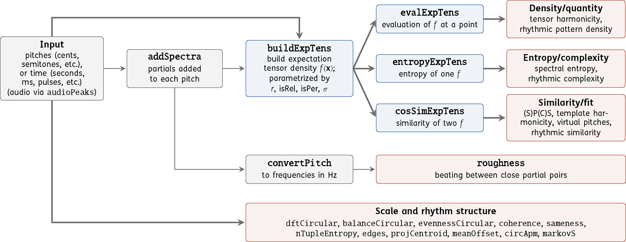
Figure 1
Dataflow through the toolbox. A weighted multiset of pitches or time points is the common input. Spectral enrichment is optional—time points bypass it, as may pitches—after which the collection becomes an expectation tensor density. Three operations are defined on a density: evaluation at a point, entropy of one, and comparison of two. Two paths bypass the density: roughness takes the partials directly, converted to Hz, and the structural measures take the weighted positions directly. Thick arrows mark the paths that serve the pitch and rhythm domains alike, with only the period changing; the thin ones pass through spectral enrichment, which applies to pitched sounds only. Colour marks each box’s role: grey for input and preprocessing, blue for the expectation tensor operations, and red for measures.
First, the domains are continuous. Pitches and time points enter as real numbers rather than as indices into a chromatic or metrical grid, so microtonal tunings, expressive timing, and spectral peaks measured from a recording are all admitted without quantization. Corpus‑ and learning‑based models of musical expectation work differently: because they typically estimate probabilities over a discrete alphabet of symbols—scale degrees, pitch classes, or categorized inter‑onset intervals—a tuning system and a metrical grid must be fixed before the analysis can begin (e.g., Pearce, 2018). Four features are exceptions, their implementations here requiring integer positions within an equal division of the period: sameness, ‑tuple entropy, the circular autocorrelation phase matrix, and Markov prediction.
Second, collections of unequal size can be compared directly. Because each multiset is embedded as a density over a shared domain before any comparison is made, no correspondence need be established between the elements of one collection and those of another. This is what distinguishes the approach from voice‑leading and related metrics, which require a matching between the two chords and so require the cardinalities to be equalized: choosing which elements of the larger collection to match against the smaller often has no unique answer, and, even where the choice is forced, the resulting distance violates the triangle inequality (Milne et al., 2011). Here, a three‑note chord and a seven‑note scale compare as readily as two triads, and a chord’s several dozen partials compare with another’s without any partial having to be paired with a counterpart.
Third, perceptual uncertainty is represented explicitly. A single smoothing‑width parameter smears each element over a range of nearby values so that near‑coincidences count in proportion to their closeness rather than being either exact matches or complete mismatches. Every measure built on the expectation tensor inherits ; among the structural features it appears in ‑tuple entropy and, as the concentration parameter of a von Mises kernel, in edge detection. Extending it to the remainder is discussed in Section 8.
Predictors drawn from different families can therefore be applied to the same stimuli within one analysis. A chord’s fit to its context and its consonance considered in isolation are different questions, and Section 5 shows that they receive close to independent answers.
Section 2 presents the expectation tensor framework, Section 3 the consonance and harmonicity measures, and Section 4 the structural features of scales and rhythms. Section 5 is an example of a worked application. Section 6 surveys prior empirical work, Section 7 describes the software design, and Section 8 discusses limitations and future directions.
2 Expectation Tensors and Their Cosine Similarity
2.1 Representing pitches and time points
The toolbox operates on collections of pitches or time points, represented as numbers. For pitch, the standard representation is a logarithmic function of frequency: , giving values in cents—a unit in which the octave spans 1200 equally spaced steps, each corresponding to 1/100 of an equal‑tempered semitone. Equal frequency ratios then correspond to equal pitch distances, so a perfect fifth (ratio 3:2) is about 702 cents in any register. For rhythmic patterns, positions are typically integers representing pulse locations within a metrical cycle (e.g., onsets at pulses 0, 3, 6, 10, and 12 within a 16‑pulse cycle for the son clave rhythm), though finer representations—such as milliseconds or subdivisions of a pulse—are also supported.
A pitch collection (or time‑point collection) is a multiset of such values—a set whose elements may repeat, such as when a chord tone is doubled by two voices. Each element may carry a non‑negative weight representing its perceptual salience, amplitude, or probability of being perceived. Multisets may be specified from symbolic data (scale degrees, MIDI note numbers, theoretical pitch sets) or extracted from audio: audioPeaks returns the frequencies and amplitudes of a recording’s spectral peaks, which convertPitch—a utility spanning seven pitch and frequency scales (Hz, MIDI, cents, mel, Bark, ERB‑rate, and Greenwood)—converts to cents for use in any toolbox function.
2.2 Definitions
The construction begins from a simple perceptual premise. A listener does not register musical events exactly: a tone is heard at a pitch that could plausibly have been any of a range of nearby pitches and with an onset at a time that could have been any of a range of nearby times—albeit more probably with values close to the true one and less probably those further away. Replacing each event by a probability distribution over nearby values, and adding these distributions together, gives a function over the domain, of pitch or of time, whose value at any point is the expected number of events perceived there (Milne et al., 2011). It is expected in the ordinary statistical sense: a value of means a listener perceives an event there in of hearings. Applied to pairs of events, it gives the expected number of ordered pairs at each combination of two positions and so on upwards. These functions are the expectation tensors.
Formally, an expectation tensor is a continuous density over ordered ‑tuples—ordered sequences of elements (an ‑ad)—drawn from a weighted multiset, each smoothed by a Gaussian kernel. ‘Tensor’ refers to the discretized form being a rank‑ array indexed by copies of the pitch or time space—a multidimensional array, not a multilinear map. The term monad denotes (individual elements), dyad denotes (ordered pairs), triad denotes (ordered triples), and so on. Given a multiset with weights , the ‑ad expectation tensor density at a query point is
where the sum ranges over all ordered ‑tuples drawn without replacement from the multiset; is the ‑th tuple (an ordered sequence of pitch values, treated as a point in ); is the product of the constituent weights; models perceptual uncertainty (for pitch, can be chosen to approximate a just‑noticeable difference; see Milne et al., 2011, Appendix A); and is a quadratic form—a function that computes a squared distance.
Two binary flags, and , together determine the mode, which fixes both the quadratic form and the dimensionality : in the absolute case and in the relative case.
Non‑periodic/Periodic (). When true, the domain is a circle of circumference (the period), with distances wrapped to . For pitch, setting implements pitch‑class equivalence; for rhythm, is the cycle length.
Absolute/Relative (). When false (absolute), the density depends on the actual positions of the elements: (the standard Euclidean squared distance, where is the difference between the query point and a tuple) and the effective dimensionality equals . When true (relative), the density is invariant under transposition—shifting all values by a constant leaves the density unchanged. This is achieved by a quadratic form , which measures distance in the subspace orthogonal to the all‑ones direction—the direction along which all elements shift together—so projecting out the mean and retaining only the intervals between elements. The effective dimensionality reduces from to , and each ‑tuple is represented by its ‑dimensional vector of intervals from one of its own elements (by convention, the first): .
The two flags yield four mode combinations, each suited to a different question. Absolute monads () give a density over individual (spectral) pitches, or pitch classes when periodic, whose entropy measures (spectral) pitch complexity (Section 2.5) and whose cosine similarity quantifies perceptual similarity (Section 2.4). Relative dyads () give a density over pairwise intervals, so comparing two such densities compares interval content—Figure 2 uses this to find which generator‑chain tunings best approximate a reference chord (Milne et al., 2011, Examples 6.3–6.5). Relative triads () give a density over interval pairs. Tensor harmonicity builds such a density from a single harmonic series and evaluates it at a triad’s own pair of intervals, thus measuring the density of that pattern within the series (Section 3.3).
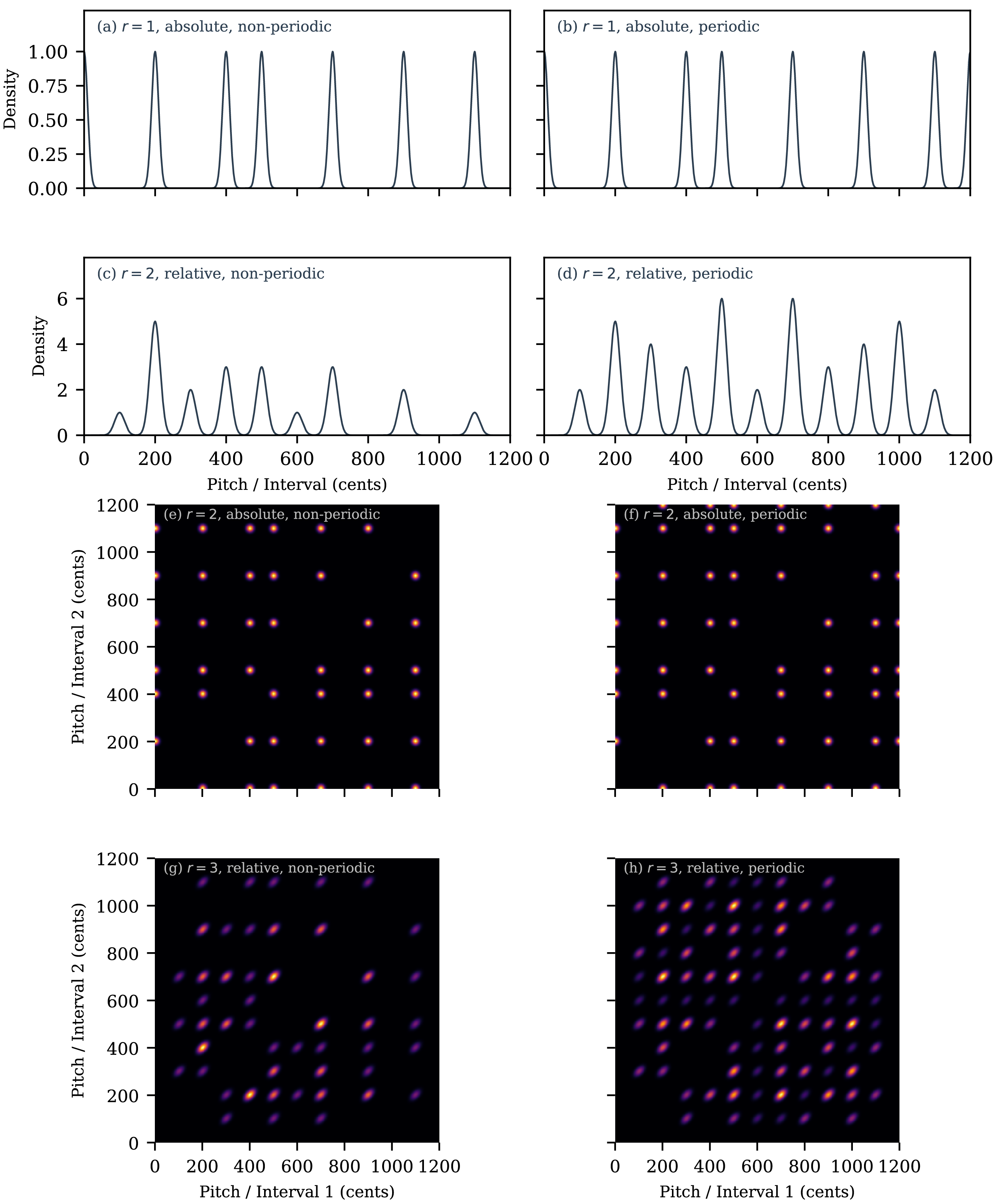
Figure 2
Spectral pitch class similarity of 20‑tone generator‑chain tunings against two reference chords: the 4:5:6 just intonation (JI) major triad (right half, red) and the 4:5:6:7 JI tetrad (left half, blue). Uniform weights; cents. With a single reference chord, each plot would have left–right reflective symmetry since generator and its complement produce the same pitch set. (a) (relative dyads; 0.1‑cent resolution): radial distance on the right indicates how closely different generator‑chain tunings approximate the pairwise intervals within the 4:5:6 triad (4:5, 5:6, 2:3); on the left, it indicates the same for the pairwise intervals within the 4:5:6:7 tetrad (4:5, 5:6, 2:3, 4:7, 5:7, 6:7). (b) (relative triads; 1‑cent resolution): the right half indicates how closely tunings approximate the 4:5:6 triad as a whole, while the left half indicates approximations to the four triads within the 4:5:6:7 tetrad (4:5:6, 4:5:7, 4:6:7, 5:6:7).
The expectation tensor framework applies equally to rhythmic patterns: the same operations, computed over time‑point multisets without spectral enrichment, yield measures of rhythmic similarity and complexity, and, evaluated at a queried pattern of onset intervals, how strongly that pattern is present in the rhythm.
Figure 3 illustrates these mode combinations by displaying the expectation tensor densities for a diatonic scale (or bembe‑12 rhythm; Undy et al., 2026) across different values of : the top two rows show one‑dimensional densities (line plots) for absolute monads () and relative dyads (), while the bottom two rows show two‑dimensional densities (heatmaps) for absolute dyads () and relative triads (). Each row contrasts the non‑periodic (left) and periodic (right) cases.
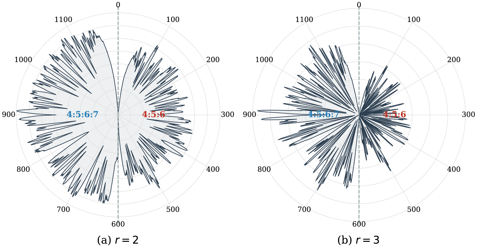
Figure 3
Expectation tensor densities for the diatonic scale ( cents, period = 1200 cents) across eight mode combinations. Left column: non‑periodic; right column: periodic. (a, b) Absolute monad (, dim = 1). (c, d) Relative dyad (, dim = 1). (e, f) Absolute dyad (, dim = 2). (g, h) Relative triad (, dim = 2). Periodic densities wrap at the octave; relative densities are transposition‑invariant. The pitch set shown is not specific to C major—any rotation of the diatonic scale yields the same relative densities and the same absolute densities up to translation.
2.3 Spectral enrichment
A notated pitch (e.g., middle C) is an abstraction: sounded on a real instrument, it produces not a pure tone but partials at approximately integer multiples of the fundamental. For symbolic input (MIDI note numbers, scale degrees, theoretical pitch sets), addSpectra appends synthetic partials to each pitch, expanding the multiset and weighting it by a spectral envelope. This is unnecessary for spectral peaks extracted from audio via audioPeaks, which already represent the full spectrum.
Five spectral modes are available—harmonic, stretched, frequency‑linear, stiff‑string, and custom—with power‑law () or geometric () weight decay, where is the harmonic number.
2.4 The pitch similarity family: (S)P(C)S
The cosine similarity of two expectation tensor densities—a standard measure of the alignment of two non‑negative functions, ranging from 0 (no overlap) to 1 (identical shape)—quantifies how similar two weighted multisets are:
where the inner product is the standard inner product: the integral, over all , of the pointwise product of the two densities. Section 2.6 shows that this integral has a closed form, so that Equation 2 can be evaluated exactly, without a grid. For expectation tensors, it also has a concrete meaning. Were perception perfectly precise, it would be the number of ordered ‑ads the two collections have in common, as a proportion of the most they could have had in common—the geometric mean of the numbers each shares with itself—and, with weights read as probabilities of being perceived, these become expected counts (Milne et al., 2011). Smoothing relaxes exact coincidence into graded near‑coincidence, which is the point of it: replacing one pitch of a major triad by a pitch 10 cents away gives a count‑based value of but a smoothed value of at cents. At with spectral enrichment, the count is the proportion of the two sounds’ partials that coincide in pitch (Milne et al., 2016).
In the pitch domain, spectral enrichment and the periodic flag yield a family of four named measures, each Equation 2 applied to a pair of densities of the form of Equation 1, differing only in two binary choices. SPCS is the most familiar: , , with , applied to multisets to which harmonic partials have been added (Milne et al., 2015). Setting gives SPS, which compares full spectra on an unbounded pitch line (Dean et al., 2019); omitting the partials gives pitch class similarity (PCS); and doing both gives pitch similarity (PS), which compares fundamentals alone (Milne et al., 2011). Enrichment is unnecessary when the input already comes from audio via audioPeaks. SPCS is the most commonly used of the four, having consistently outperformed SPS at modelling perceived tonal fit, which is attributed to the perceptual importance of octave equivalence (Milne et al., 2015).
Where no additional information about the experimental stimuli is available, suitable values are 12–24 harmonics, power‑law rolloff , and between about 6 cents (Milne et al., 2015; Milne and Holland, 2016) and 10 cents (Hearne et al., 2026). (The figures and analyses in this article use cents, 16 harmonics, and unless stated otherwise.) When experimental conditions are known (e.g., a specific instrumental spectrum), parameters can be matched to those conditions; for example, Hearne et al. (2026) fit to the spectral rolloff of their stimuli. Figure 4 illustrates SPCS profiles for two contrasting scales; Figure 5 shows SPCS for all triads containing a perfect fifth, relative to major and minor reference triads, illustrating the differential similarity structure of the two modes.
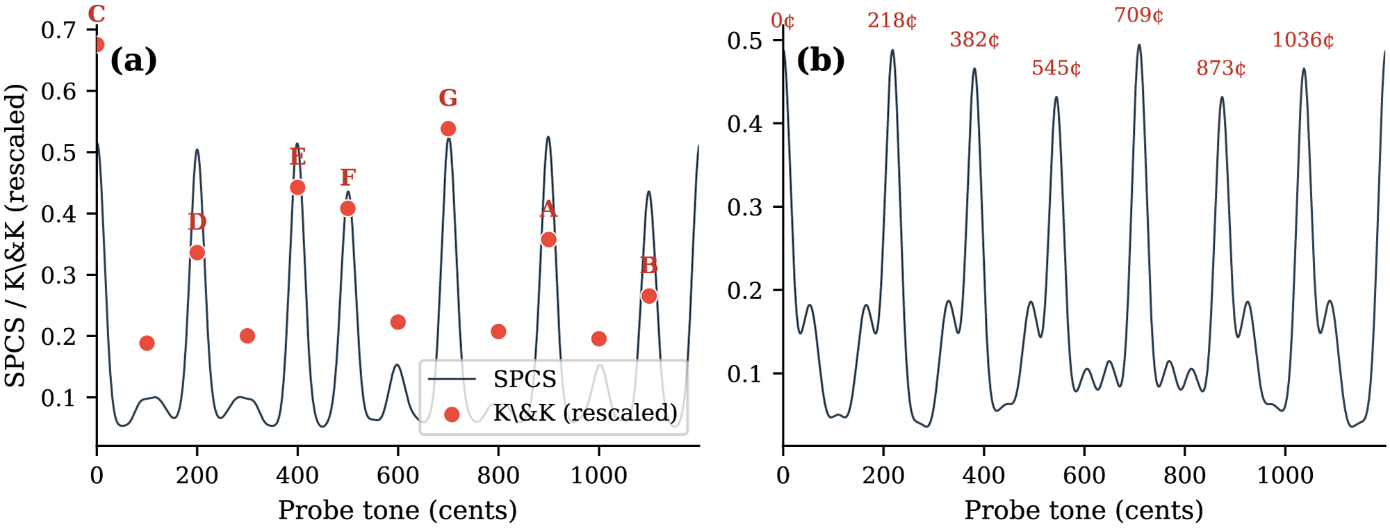
Figure 4
Spectral pitch class similarity (SPCS) of probe tones against two reference scales. (a) C major scale in 12‑TET, with Krumhansl and Kessler’s (1982) empirical probe‑tone ratings (red dots, affinely rescaled to minimize squared error with SPCS values at the 12 semitone positions; with these parameters). (b) Porcupine[7] scale in 22‑EDO (step pattern 4333333) suggesting a psychoacoustically motivated major tonic on the scale’s first degree and minor tonic on its fifth degree. (EDO stands for equal divisions of the octave.)
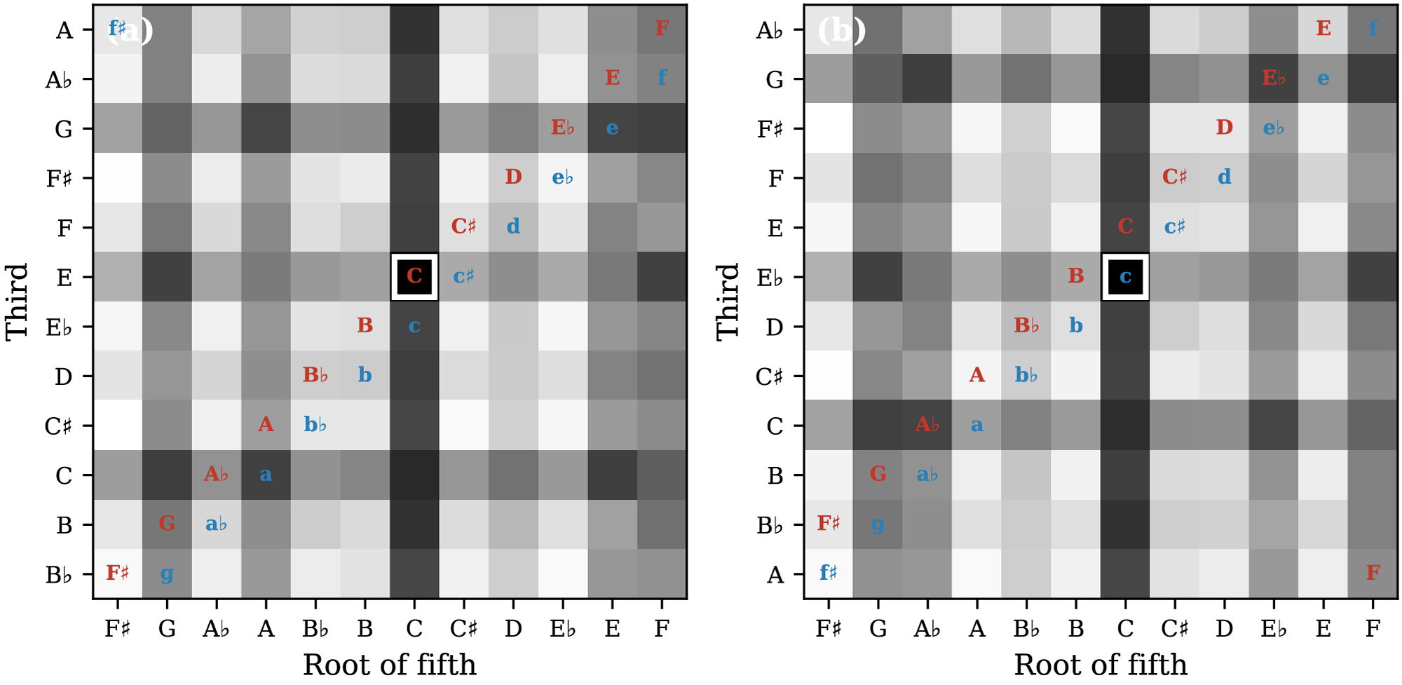
Figure 5
Spectral pitch class similarity of all 12‑EDO triads comprising a perfect fifth relative to (a) a C major reference and (b) a C minor reference. Major triads are labelled in red, while minor ones are labelled in blue; the white square marks the reference. Darker cells indicate greater similarity.
2.5 Entropy of expectation tensors
In addition to cosine similarity, the toolbox computes the Shannon entropy of expectation tensor densities via entropyExpTens. The entropy of a density quantifies its disorder: a density concentrated at a few sharp peaks has low entropy, while a diffuse one has high entropy. This gives a complexity measure applicable to any tensor mode and any domain.
The entropy of a relative periodic dyad tensor (, , ), for example, quantifies the complexity of a pitch set’s interval content: intervals clustering at a few values, as in an equal‑tempered scale, give low entropy; many distinct intervals give high. Spectral entropy (Section 3.1) is one application of this idea—the entropy of a spectrally enriched absolute non‑periodic monad tensor—and higher‑order tensors capture correspondingly higher‑order regularities.
Because the differential entropy of a Gaussian mixture has no known closed form—the logarithm of a sum of Gaussians does not simplify—entropy is computed on a grid, unlike cosine similarity.
2.6 The analytical inner product
Evaluating Equation 2 requires the inner product of two densities of the form of Equation 1. Because a product of Gaussians is itself Gaussian, that integral has a closed form:
where denotes the ordered ‑tuples of a collection and its unordered ‑subsets. Because is unchanged by permuting the elements within both tuples together, only one side need be ordered; taking combinations on the other is cheaper by a factor of . The omitted proportionality constant depends only on and , and is common to all three inner products in Equation 2, so it cancels and the cosine similarity follows directly—a finite double sum over tuples, with no discretization, grid, or resolution parameter and exact to floating‑point precision. This result is due, in its original form, to David Bulger (personal communication, 2016) and was implemented for the cosine similarity in version 1 of the toolbox. Its derivation, for all four modes and including the additional wrapping the relative periodic case requires, is given in the Supplementary Material.
Version 1 instead built the densities themselves on a discrete grid of rounded pitches, an approach that imposes a resolution parameter, rounds every input, and grows with the size of the domain raised to the tensor order: an absolute triad tensor over the octave occupies some elements and only was implemented. The analytical form has none of these costs and scales with the number of elements in the collection rather than the size of the domain.
3 Consonance and Harmonicity
Musical sounds can be perceived as consonant (pleasant, stable, harmonious) or dissonant (unpleasant, tense, rough)—a perceptual dimension that has been studied since antiquity. Contemporary models distinguish at least three contributing factors (Eerola and Lahdelma, 2021; Harrison and Pearce, 2020): roughness (the rapid amplitude fluctuation produced by close‑frequency partials interfering in the auditory system), harmonicity (the degree to which a chord’s intervals or composite spectrum align with a harmonic series), and familiarity (the degree to which a musical structure matches culturally learned expectations).
The toolbox implements models of the first two factors. It does not model familiarity, which requires corpus‑based or learning‑based approaches such as IDyOM (Pearce, 2018). The toolbox’s spectral entropy measure (Section 3.1) does not fit neatly into any of these three categories—it captures a distinct aspect of spectral complexity that is related to, but not reducible to, either roughness or harmonicity.
The five measures respond to different properties of a chord and each subsection below notes what its measure is most and least sensitive to. Four properties are distinguished: type, the pitch‑class set; inversion, which chord tone lies lowest; spacing, the pitch range the chord spans; and register, its mean pitch. The sensitivities reported are shares of rank variance over 162 chords crossing six types—from the major triad to a semitone cluster—with three inversions, three spacings, and three registers, spacing and register varied independently of one another.
3.1 Spectral entropy
Spectral entropy (Milne et al., 2017; Smit et al., 2019) measures the Shannon entropy of a chord’s composite spectrum after Gaussian smoothing. As noted in Section 2.5, this is one specific application of the general entropy‑of‑tensor framework: it is the entropy of an absolute non‑periodic monad expectation tensor density (with spectral enrichment applied). The underlying intuition is one of spectral concentration. Each tone of the chord contributes a series of partials; where partials from different tones land on the same pitch they reinforce one another, and the composite spectrum consists of a few tall peaks separated by empty regions. Where they land on many distinct pitches the spectrum is spread thinly and evenly. Entropy measures exactly this contrast, being low for the concentrated case and high for the diffuse one. It thus approximates the aggregation of all pairwise spectral pitch similarities within a chord, and so models the mutual fit of its tones (Milne, 2024; Milne et al., 2017). Unlike SPCS, which compares two pitch sets, spectral entropy is a property of a single (potentially composite) set. It responds mainly to spacing (0.70) and much less to type (0.17) or inversion (0.01); because the spectrum is referred to its own lowest pitch, register has no effect at all.
3.2 Template harmonicity
Template harmonicity (templateHarmonicity; Milne, 2013; Milne et al., 2016) cross‑correlates a chord’s composite spectrum with a harmonic template. The procedure is: (1) construct the chord’s absolute non‑periodic monad density (its composite spectrum), (2) construct a single harmonic template—the absolute non‑periodic monad density of one complex tone at 0 cents with harmonics, (3) evaluate both densities on a fine grid, and (4) normalize and cross‑correlate.
Informally, the procedure slides a single harmonic series along the pitch line and asks, at each position, how well its partials line up with the chord’s. A chord that is close to a segment of one harmonic series will align well at the position of that series’ fundamental and poorly elsewhere, giving a profile with one dominant peak; a chord that is not will align moderately at several positions. Two summary statistics are extracted: , the maximum of the normalized cross‑correlation (Milne, 2013), which is the cosine similarity at the best‑matching transposition, and , the entropy of the cross‑correlation profile (Harrison and Pearce, 2020), which captures whether the chord has one clear virtual fundamental or several competing ones. Both are transposition‑invariant—transposing the chord merely shifts the cross‑correlation profile, leaving its maximum and its entropy unchanged—and so unaffected by register. Otherwise, they diverge: is the most type‑sensitive of the five measures (0.67), whereas responds to type (0.52) and spacing (0.34) alike. These last two shares are the only ones in this section much affected by the number of harmonics in the template: with 24 rather than 16, they become 0.31 and 0.57, reversing their order.
The related function virtualPitches returns the full cross‑correlation profile, whose peaks indicate candidate fundamentals—the pitches the auditory system infers from a complex of partials (Parncutt, 1988). The template’s spectral rolloff alters the number and prominence of those peaks.
3.3 Tensor harmonicity
Tensor harmonicity (tensorHarmonicity; Smit et al., 2019) measures how probable a chord’s specific ordered intervals are within a single harmonic series.
In the counting terms of Section 2.4, tensor harmonicity is the expected number of ordered ‑ads of partials, drawn from a single harmonic series, whose interval pattern is the chord’s own: where the cosine similarity counts the ‑ads that two collections share, this counts the ‑ads of one collection matching a single query pattern, with again letting near‑coincidences contribute. Some patterns recur throughout the series and others hardly do at all—the major triad’s intervals, given by 4:5:6 and its multiples, are common; the minor triad’s, 10:12:15, far less so. A chord need not be justly tuned to score well, however. Figure 6a magnifies the landscape around the triads of common practice: the equal‑tempered major triad in root position lies 13.7 cents from the just‑intonation 4:5:6 triad in one interval and 2.0 cents in the other, displacements comparable to itself, and so sits within that peak rather than outside it. Because the pattern is measured from the lowest tone upwards, the answer depends on how the chord is voiced and not only on which pitch classes it contains. Like , it is driven more by type (0.26) than by spacing (0.17), and, the density being relative, register does not move it at all. It also leaves most of its variance unexplained by any of the four properties singly (0.54), its responses to inversion and spacing depending on the chord type. Figure 6 shows this dependence directly, and it is what produces the distinctive topography of Figure 7c.
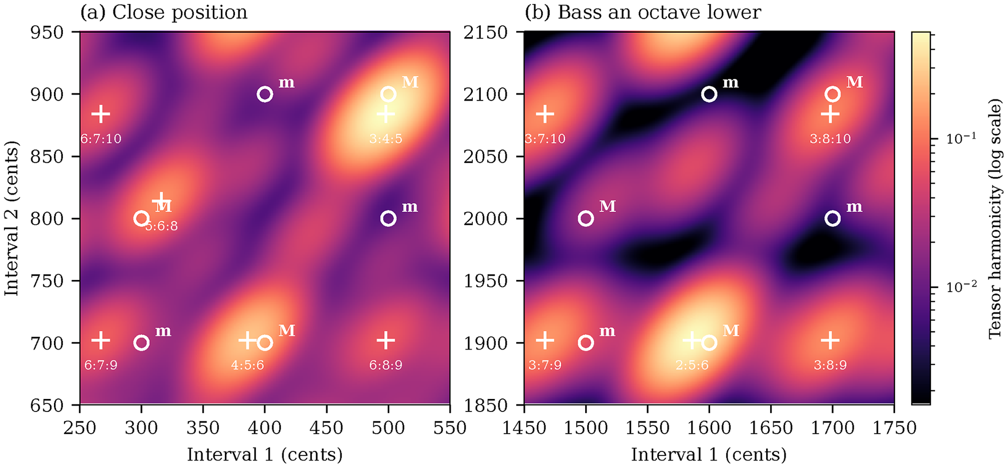
Figure 6
Tensor harmonicity across two regions of the triad landscape, at 1‑cent resolution, with for cents as in Figure 7c, at the article’s 16 harmonics per tone. Open circles mark the six 12‑EDO voicings, major (M) and minor (m) in root position and first and second inversion; crosses mark the local maxima, labelled with the simplest integer frequency ratio that produces each. (a) Close position, where the second inversion scores highest. Note that the just minor triad 10:12:15 is not itself a maximum, lying between peaks, whereas the subminor 6:7:9 to its left is one. (b) The same six chords with the bass an octave lower, where root position scores highest instead. Colour is logarithmic, for legibility only: which transformation of the density best reflects perception is an open question.
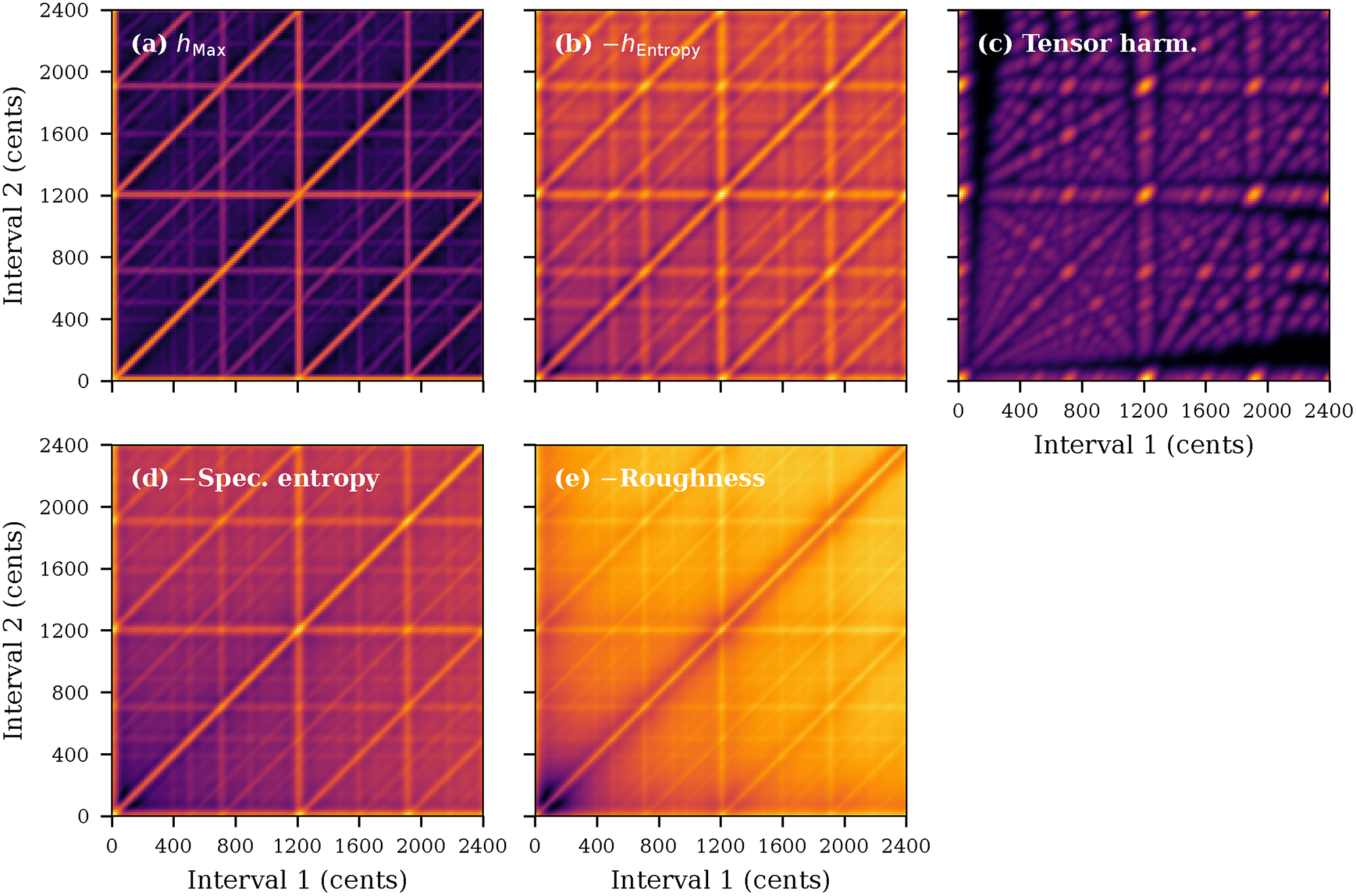
Figure 7
Five consonance‑related measures for triads with both intervals swept from 0 to 2400 cents. Brighter regions indicate higher consonance (roughness and spectral entropy are negated so that peaks correspond to consonance in all panels). Here, cents, the value used for spectral entropy and template harmonicity in Milne et al. (2023b); tensor harmonicity uses , for the reason given in Section 3.3. Note the distinctive topography of tensor harmonicity (c) compared to the other measures. (Different gamma compressions have been applied to ensure the visibility of low‑level features.)
Concretely: a harmonic template is built with the template pitch (0 cents) duplicated times before harmonics are added, where is the chord cardinality; the relative ‑ad expectation tensor of that template is constructed; and it is evaluated at the chord’s ordered interval vector, i.e., the intervals from its lowest tone to each of the others. The duplication is what allows unisons to count as consonant: without it, each position in a tuple must be filled by a different partial, so no partial can contribute to more than one position. The ordered vector distinguishes chords of identical unordered interval content—the major triad and the minor both contain the intervals , but their ordered vectors are and . Because the chord enters only as a query point, its own perceptual uncertainty is not otherwise represented. Folding it in amounts to integrating the density against a second Gaussian, which is exactly equivalent to widening the template’s kernel: for uncertainties on the template and on the query, the width becomes , or when the two are equal.
3.4 Roughness
Sensory roughness (roughness) computes the beating‑based dissonance of close partial pairs using Sethares’s (1993) parameterization of Plomp and Levelt’s (1965) empirical dissonance curve.
The implementation extends the original model in two ways. First, pairwise roughnesses are combined via a configurable ‑norm (default , a simple sum). Kameoka and Kuriyagawa (1969) and Hutchinson and Knopoff (1978) used different aggregation methods—the former a compressive power law, the latter an amplitude‑weighted average—and both approaches have known limitations (Mashinter, 2006; Parncutt, 2006). The ‑norm allows these and other aggregation methods to be explored: higher gives greater weight to the roughest pairs. Second, optional averaging over the partial pairs gives the expected roughness of a randomly chosen pair, making values comparable across chords with different numbers of partials.
Unlike the other measures, roughness is register‑dependent and so requires frequencies in Hz: the same interval is rougher in lower registers where partials are more closely spaced on the basilar membrane. It is alone in responding to register (0.33), and responds far more to spacing (0.48) than to type (0.09)—though the type effect is real, a semitone cluster being markedly rougher than any triad at the same spacing and register.
Figure 7 compares all five consonance‑related measures across a two‑octave space of triads.
4 Scale and Rhythm Structure
The toolbox provides functions for computing structural and perceptual features of sets of points distributed around a circle. These apply equally to pitch‑class sets (where the circle is one octave) and to time‑class sets (where the circle is one rhythmic cycle).
4.1 Fourier‑based measures
The discrete Fourier transform (DFT) of a set of weighted points on a circle (dftCircular) is computed directly from the point positions, in two steps. Each of the points , carrying weight on a circle of circumference , is first mapped to the complex number , whose argument is the point’s angular position and whose modulus is its weight. The points are then sorted by position and an ordinary length‑ DFT is taken over this sequence of complex numbers, giving coefficients .
The low‑order coefficients have direct interpretations. The zeroth, , is the sum of these complex numbers, so that locates the set’s centre of gravity: greatest when the points cluster to one side of the circle, and zero when that centre of gravity coincides with the circle’s own. The first, , is large when successive points are separated by a constant angle, since a constant separation of is exactly the rotation that the first DFT basis vector removes. Balance and evenness, defined below, report these two quantities. Weights have a clear meaning only in the zeroth coefficient, where they scale each point’s contribution to the centre of gravity. Coefficients beyond the first have less obvious interpretations but may nonetheless be perceptually relevant; their potential role is explored in Milne and Herff (2020) and its Supplementary Material.
This construction is distinct from the more common approach in mathematical music theory, where sets are represented as binary indicator vectors—vectors of 0s and 1s over a discretized grid—and the DFT is computed from this indicator (e.g., Amiot, 2016; Quinn, 2007), giving one coefficient per grid position. The direct approach accommodates non‑integer positions and weighted events without discretization.
Balance (balanceCircular; Milne et al., 2017) measures how close a set’s centre of gravity is to the circle’s centre and is defined as . It ranges from 0 (all weight at a single point: the centre of gravity is maximally far from the centre) to 1 (the centre of gravity lies exactly at the centre).
For example, in a 12‑step chromatic universe: the augmented triad has balance 1.000, the major triad has balance 0.827, and the cluster has balance 0.089 (see Figure 8).
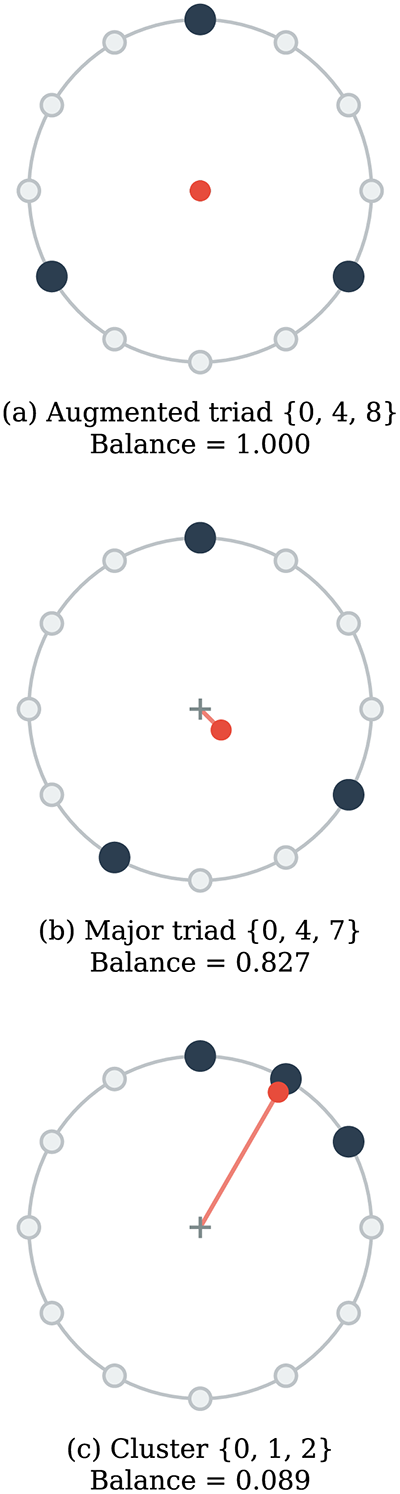
Figure 8
Balance illustrated on the chromatic circle. Filled circles mark pitch classes in each set; the small red circle shows the centre of gravity of the set, and the red line connects it to the circle’s centre. (a) The augmented triad is perfectly balanced: its centre of gravity lies at the centre. (b) The major triad is nearly balanced. (c) The cluster is highly unbalanced: its centre of gravity is far from the centre.
A perfectly balanced set—one with balance exactly 1—need not be evenly spaced or regular. Any union of isochronous cycles is perfectly balanced—a three‑against‑four cross‑rhythm, for instance—and stays so when the cycles are rotated independently of one another so that no two events coincide. Others arise only when a negatively weighted cycle is added whose every event coincides with, and so annihilates, an event of the positive ones: nothing negative survives, but the pattern left behind could not have been assembled from positive cycles alone. Such patterns are neither regular nor decomposable into smaller balanced parts and are distinct from the familiar well‑formed (moment‑of‑symmetry) and maximally even classes (Milne et al., 2017).
Evenness (evennessCircular; Milne et al., 2017) is the normalized magnitude of , computed with uniform weights. It ranges from 0 to 1, equalling 1 only for equally spaced sets.
For example, the whole‑tone scale has evenness 1.000, the diatonic scale has evenness 0.989, and a maximally clustered set like has evenness 0.644.
4.2 Interval‑structure measures
The following functions characterize the interval structure of a set of points on a circle. Coherence accepts positions at any resolution (integer or float); the implementations of sameness and ‑tuple entropy require integer positions within an equal division of the period (e.g., the 12 pitch classes of 12‑tone equal temperament or the 16 pulses of a 4/4 bar subdivided into semiquavers). More detailed descriptions of these features, including formal definitions, are available in Milne et al. (2023a).
Coherence (coherence; Balzano, 1982; Carey, 2002; Rothenberg, 1977) measures how consistently the ordering of intervals by generic span—the number of scale steps between two events—matches their ordering by specific size—the actual distance between them. A scale is coherent when a larger generic span always implies a larger or equal specific size. Failures are of two kinds: an ambiguity, where the two intervals have the same specific size, and a contradiction, where the larger generic span is strictly the smaller interval. The diatonic scale in a 12‑step universe has coherence quotient 0.993, its single failure an ambiguity: the augmented fourth F–B spans three generic steps and the diminished fifth B–F spans four, yet both measure six semitones. The blues scale scores 0.600, and its failures include contradictions: F–G spans two generic steps but measures two semitones, fewer than the three of C–E, which spans one.
Sameness (sameness; Carey, 2002; Carey, 2007) counts a set’s ambiguities alone, reporting one minus that count as a proportion of the most a set of its size could have. The blues scale therefore scores 0.787 where its coherence was 0.600, the gap being its 10 contradictions; the diatonic scale, having none, scores 0.992 against 0.993.
‑tuple entropy (nTupleEntropy; Milne and Dean, 2016) computes the Shannon entropy of the distribution of consecutive step‑size sequences of length . When , this is the step‑size (IOI) entropy; 1‑tuple entropy was empirically validated as a predictor of rhythmic recognizability and liking in Milne and Herff (2020) and applied theoretically as a measure of scale‑step complexity in Milne (2024). Higher values indicate less regularity among the sequences of adjacent steps. For example (1‑tuple entropy), the diatonic scale has 1‑tuple entropy of 0.863 bits (two step sizes: 1 and 2, in a 5:2 ratio), the chromatic scale has 1‑tuple entropy of 0.000 bits (one step size), and the son clave in 16 has 1‑tuple entropy of 1.522 bits (three step sizes: 2, 3, and 4). At , the distribution is over adjacent pairs of steps: the diatonic scale’s seven pairs are three times and and twice each, giving 1.557 bits.
Well‑formed patterns minimize ‑tuple entropy over all other arrangements of the same steps. Gaussian smoothing is optionally available, incorporating perceptual uncertainty as elsewhere in the toolbox.
4.3 Position‑level features
The following functions return values at every position around the circle. Edges, projected centroid, and mean offset accept event positions at any resolution and evaluate at arbitrary query points; the implementations of the circular autocorrelation phase matrix and Markov prediction require integer event positions. More detailed descriptions are available in Milne et al. (2023a). Figure 9 illustrates all five for the son clave rhythm.
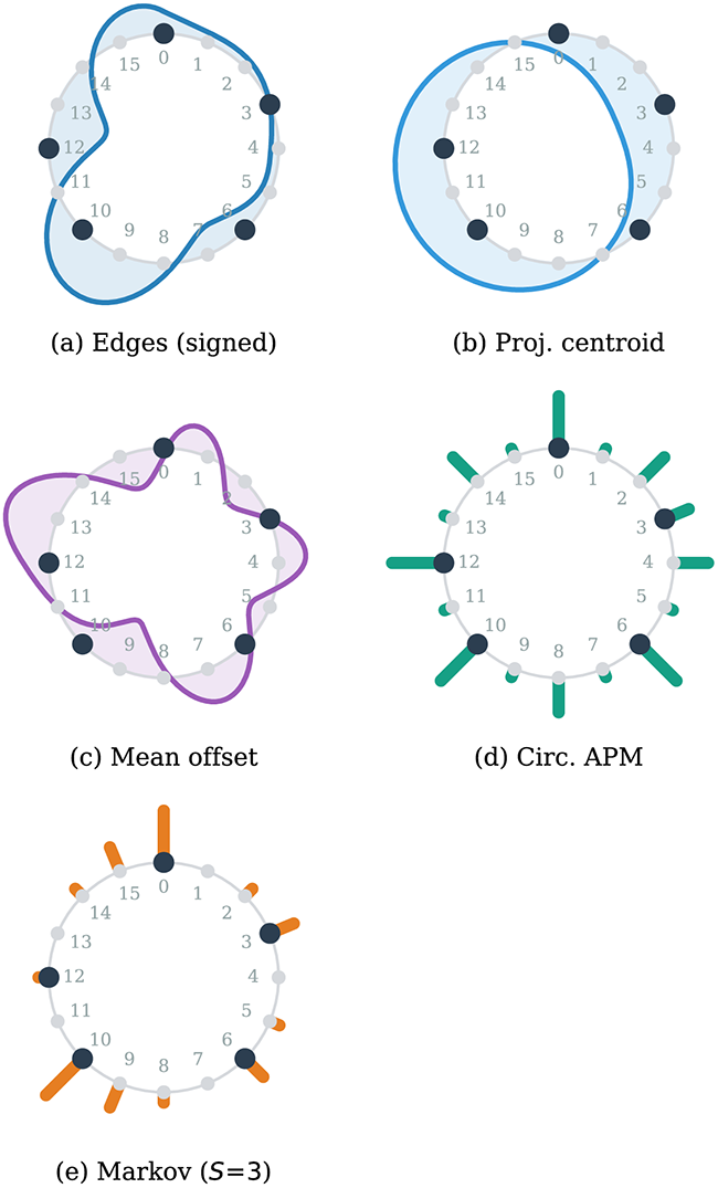
Figure 9
Five position‑level features for the son clave rhythm in a 16‑step cycle. Event positions are marked by filled black circles; position 0 is at 12 o’clock and positions proceed clockwise. Smooth curves (a–c) show continuous features; bars (d, e) show discrete features. Each panel is scaled radially to its own maximum absolute value. (a) Signed edges (): positive values (outward) mark transitions from sparse to dense; negative (inward) mark them from dense to sparse. (b) Projected centroid: near zero throughout (maximum magnitude 0.016, against 1 for a single event) reflecting the pattern’s near‑perfect balance. (c) Mean offset. (d) Circular APM (summed across lags). (e) Markov prediction ().
Edge detection (edges; Milne et al., 2023a) identifies sharp transitions between event‑dense and event‑sparse regions of the cycle. It uses the analytic first derivative of the von Mises distribution—the circular analogue of the Gaussian—namely, , whose concentration parameter sets the spatial scale: larger detects finer transitions.
In the son clave in a 16‑step cycle, large positive values appear at positions 9–10, where the gap at 7–9 gives way to events at 10 and 12, and large negative values at positions 12–13, where events give way to the next gap.
Projected centroid (projCentroid; Milne et al., 2023a) projects the circular centre of gravity onto each angular position, giving a position‑level generalization of the set‑level balance measure.
Mean offset (meanOffset; Milne et al., 2023a) computes, for each position, the net upward arc to all events. For pitch classes, this formalizes and generalizes Huron’s (2008) average pitch height, returning a value at every position and so capturing how ‘bright’ or ‘dark’ a mode sounds from any chromatic vantage point. The related concept of mode height is used by Hearne (2020) and Tymoczko (2023).
For example, in the diatonic scale: the Lydian mode (starting on pitch class 5) has the highest mean offset (brightest), while the Locrian mode (starting on pitch class 11) has the lowest (darkest).
Circular autocorrelation phase matrix (circApm; Milne et al., 2023a) adapts Eck’s (2006) autocorrelation phase matrix (APM) to the periodic case. Standard autocorrelation reveals which periodicities are present but discards phase information; the APM preserves it by storing, for each lag , the autocorrelation energy indexed by phase position so that peaks indicate events recurring at specific intervals from specific phases.
For example, summing across lags assigns each position of the son clave a weight reflecting how strongly it participates in the pattern’s periodic structure. Positions 0, 6, 10, and 12 score highest, sitting on the clave’s dominant even‑lag periodicities, while position 3 scores roughly half that despite carrying an event; non‑event positions score above zero where they align with the underlying structure.
Markov prediction (markovS; Milne et al., 2023a; originally by David Bulger) predicts the event weight at each position from the positions preceding it. Positions whose preceding patterns of events and non‑events are identical form a group, and each is assigned that group’s mean event weight. The result is the optimal ‑th order Markov predictor for the cycle; with binary weights, it is the proportion of a group’s positions that carry an event, and so a probability.
For example, in the son clave with , positions 0 and 10 are each preceded by three consecutive non‑events, and, as both carry an event, each takes a predicted value of 1. Positions 2, 5, 8, 12, and 14 are each preceded by non‑event, event, non‑event; only one of the five, position 12, carries an event, so each takes a predicted value of 0.2.
5 A Worked Application
This section applies the toolbox to a concrete stimulus set: chordal probes heard against a tonal context. Each probe is characterized both by its similarity to the context and by its consonance in isolation, using measures from Sections 2 and 3. All values are reproducible with the scripts archived at https://doi.org/10.17605/OSF. IO/2K6TD.
5.1 Stimuli
The context is a four‑part I–IV–V7 progression in C major, voiced C3–G3–E4–C5, F2–A3–F4–C5, G2–D4–F4–B4. The context is presented to the measures as the union of the three chords, a 12‑element multiset.
The probes are triads on four scale degrees—the tonic and submediant, which are diatonic to the context, and IV and II, which are not—in three qualities (major, minor, diminished) and three inversions, giving 36 probes. Each is voiced in four parts, and the voice leading throughout—within the context, and from the V7 to each probe—follows conventional rules, so spacing varies across the probe set rather than being held fixed.
5.2 Predictors
A probe’s contextual fit—how well it accords with the progression—is quantified by the four measures of Section 2.4: SPCS, SPS, PCS, and PS. Its intrinsic consonance is quantified, without reference to the context, by tensor harmonicity, , , spectral entropy, and roughness. The fit measures use cents, as in Hearne et al. (2026); the consonance measures use cents, as in Milne et al. (2023b), with tensor harmonicity at for the reason given in Section 3.3. Roughness is computed on frequencies in Hz and averaged over partial pairs. The measures are on different scales, and which transform of a raw density best reflects perception is an open question, so the correlations below are Spearman, unaffected by any monotone rescaling.
5.3 Results
SPCS ranges from for the tonic triad down to for IV major and correlates at with PCS and with SPS. PS correlates least with the others ( with SPCS); without partials, it counts coincident pitches, just as PCS counts coincident pitch classes.
Figure 10 shows the relation between the two families. Within the fit block, correlations range from to , and, within the consonance block, range from to ; across the two blocks, none exceeds in magnitude. Two pairs illustrate this. The tonic and II minor triads, both in second inversion, are all but identical in consonance ( against , spectral entropy against ) yet differ nearly fourfold in fit ( against ). Conversely, IV minor in first inversion and II major in root position fit the context almost equally well ( against ) while differing sharply in consonance ( against , and tensor harmonicity against ). No comparison requires equal cardinality: each probe has four tones, the context 12.
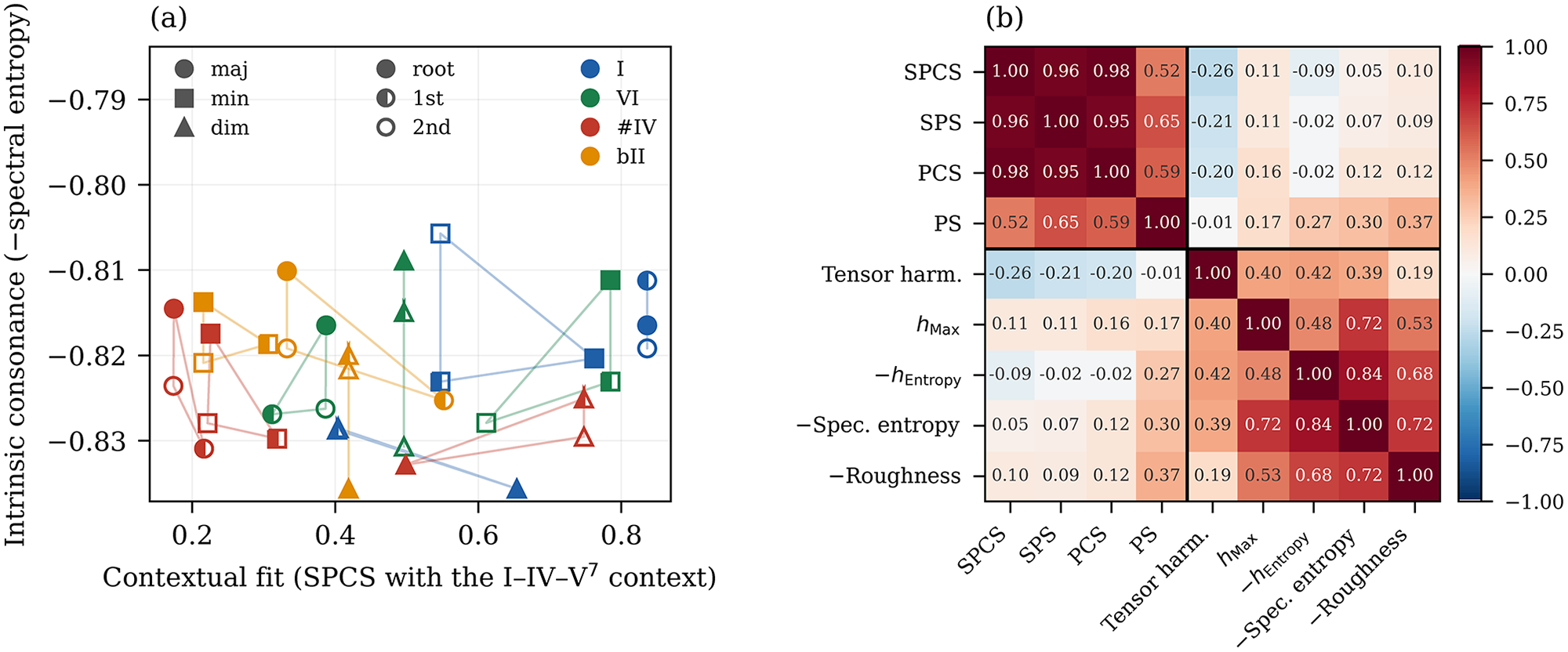
Figure 10
The worked application of Section 5. Entropies and roughness are negated throughout, so that every measure increases with consonance. (a) The 36 probes plotted by fit to the context against intrinsic consonance (spectral entropy). Marker shape gives chord quality, fill gives inversion, colour gives the root, and faint triangles join the three inversions of each chord. Since no two probes are transpositions of one another, the vertical spread reflects quality and voicing rather than the root, to which spectral entropy is invariant. (b) Spearman rank correlations among the nine predictors; the rule separates the fit measures from the consonance measures.
A study predicting responses to chords in context therefore needs predictors from both families since neither carries the other’s information: the contextual (‘horizontal’) and simultaneous (‘vertical’) aspects of musical stability are separately necessary (Hearne et al., 2026; Tenney, 1988).
6 Prior Empirical Applications
The measures implemented in the toolbox have been tested against behavioural data in a range of music perception experiments. This section surveys the principal findings.
6.1 Tonal fit and tonal hierarchies
SPCS was introduced as a model of tonal hierarchy in Milne et al. (2015), where it was fitted to Krumhansl and Kessler’s (1982) probe tone data—ratings of how well each of the 12 chromatic pitches fits a previously established major or minor context. Cross‑validated correlations were high ( for the best variant), using harmonic complex tones with a rolloff and cents. It extends to predicting the tonics of harmonic minor, melodic minor, and harmonic major scales and of microtonal scales for which no empirical data then existed.
Milne et al. (2016) tested SPCS with microtonal melodies and inharmonic spectra. Participants chose which of two melodies—one tuned to match the inharmonic spectrum, the other mismatched—was more ‘natural.’ A logistic regression combining SPCS and template harmonicity significantly predicted their choices.
Milne and Holland (2016) used SPCS to predict perceived triadic distance, finding it outperformed voice‑leading models and predicted a pitch space close to the music‑theoretical Tonnetz. Homer et al. (2024) developed a related spectral model, influenced by SPCS, with broadly comparable performance on the probe tone data.
Hearne et al. (2026) examined tonal hierarchies in microtonal scales (22‑EDO) as well as familiar and unfamiliar 12‑EDO scales, using both ‘fit’ and ‘stability’ as rating terms. SPCS was a strong predictor of ratings for unfamiliar scales—for which corpus‑based predictors (pitch prevalence) are, by definition, unavailable—supporting the claim that acoustical features play a foundational role in tonal function.
6.2 Consonance and affect
Harrison and Pearce (2020), in a large‑scale computational study of simultaneous consonance, introduced the summary statistic extracted from the SPCS cross‑correlation profile (here implemented in templateHarmonicity). Eerola and Lahdelma (2021) evaluated multiple acoustic and cultural predictors of consonance across several published datasets, finding that harmonicity (specifically, the measure of Harrison and Pearce, 2020) and roughness were among the strongest predictors.
Smit et al. (2019) used roughness, spectral entropy, and tensor harmonicity to predict pleasantness and happiness/sadness ratings for chords in the Bohlen–Pierce tuning system—a non‑octave tuning unfamiliar to all participants. Spectral entropy (introduced theoretically in Milne et al., 2017) and tensor harmonicity (introduced theoretically in Smit et al., 2019) were both tested against empirical data for the first time, and all three measures were significant predictors in the expected directions. Further theoretical predictions using spectral entropy—without empirical validation—were subsequently made in Milne (2024).
6.3 Scale and rhythmic structure
Milne and Herff (2020) tested balance, evenness, and 1‑tuple (IOI) entropy as predictors of rhythmic recognizability and liking across a large number of complex rhythms; all three were strongly evidenced.
Milne et al. (2023a) extended this to tapping accuracy, testing a comprehensive set of structural predictors—including edges, projected centroid, mean offset, circular autocorrelation phase matrix, and Markov prediction—against tapping data for a wide variety of long and complex rhythms. Entered into a Bayesian multilevel regression, they explained a substantial proportion of variance in tapping accuracy, with edge detection, projected centroid, and Markov prediction the strongest individually.
Average pitch height—which mean offset formalizes and generalizes—has been tested as a predictor of the perceived emotional valence of diatonic modes. Temperley and Tan (2013) found that perceived happiness of modes generally increases with average pitch height (the Lydian mode bucking this trend, presumably due to other factors). Smit et al. (2022) tested mean pitch as a predictor of perceived happiness cross‑culturally, comparing responses from participants in Sydney and remote communities in Papua New Guinea; mean pitch was a significant predictor for Sydney participants, though the evidence for a universal effect was negligible.
7 Software Design
The expectation tensor core is organized around precomputed density objects: buildExpTens computes all tuple indices, pitch matrices, and weight products into a struct (MATLAB) or dataclass (Python) that is reused across calls to evalExpTens and cosSimExpTens, avoiding recomputation. All functions follow a consistent API with pitches and weights as the first two positional arguments.
All functions are available in both MATLAB (camelCase) and Python (snake_case) with identical semantics, producing the same outputs to floating‑point precision (audioPeaks excepted, whose output may differ slightly between platforms). The Python implementation is installable via pip and accessible from a single namespace (import mpt). Nine demo scripts in each language cover the main use cases—an overview, and one each for audio analysis, batch processing, equal‑division approximation, expectation tensor plots, generator‑chain similarity, triad consonance, triad similarity grids, and virtual pitches; the Python demos are also provided as Jupyter notebooks. A user guide documents every function and works through its use.
8 Discussion
Five limitations and directions for future work are worth noting. First, the expectation tensor framework uses a locally Euclidean metric. For any logarithmic frequency scale (such as cents or semitones), this provides approximately uniform perceptual spacing and is well justified for periodic representations, where the domain spans a single octave. For non‑periodic representations spanning wider frequency ranges, however, pitch uncertainty is not perfectly uniform on the log‑frequency scale—it varies with register. Psychoacoustically established scales such as ERB‑rate accommodate this variation, providing more uniform perceptual spacing across the full frequency range.
In one dimension, this is straightforward: convert to the desired psychoacoustic scale before calling the toolbox so that a fixed has the correct perceptual width at all frequencies. In higher dimensions (), a Riemannian (position‑dependent) metric would be needed to scale appropriately at all pitch combinations—a direction for future development.
Second, the relationship between tensor harmonicity and other consonance measures merits further investigation. Its distinctive topography, and its low correlation with the other consonance measures (Section 5) despite all four being grounded in spectral relationships, suggest it captures a genuinely different aspect of the percept. The relation to Erlich’s harmonic entropy (Sethares, 2005), which approaches a similar question from number‑theoretic foundations, is likewise unexplored.
Third, while empirical work has focused on absolute monad similarities (the (S)P(C)S family), the toolbox supports higher‑order and relative similarities and entropies capturing interval‑level regularities. These remain largely unexplored empirically.
Fourth, the Fourier‑based measures implemented here use only the zeroth coefficient (balance) and first coefficient (evenness), but higher‑order DFT coefficients capture finer distributional structure—for example, the second coefficient relates to dyadic regularity, the third to triadic, and so on. Preliminary evidence suggests that these higher‑order coefficients may also have perceptual relevance (Milne and Herff, 2020), but systematic empirical investigation is needed.
Fifth, the position‑dependent structural features (edges, projected centroid, mean offset) operate on crisp event positions. Adding Gaussian smoothing—analogous to in the expectation tensor framework—would let them incorporate pitch or temporal uncertainty, bringing them into line with the perceptually motivated design of the tensor‑based measures.
It is hoped that the improved documentation, consistent API, dual‑language availability, and demo scripts of Version 2.0 will lower the barriers to adoption in music cognition research and MIR applications.
Acknowledgements
The analytical inner product presented in Section 2.6 is due, in its original form, to David Bulger, who also devised the Markov prediction feature of Section 4.3.
Funding Information
This work was supported, in part, by an Australian Research Council Discovery Early Career Researcher Award (project no. DE170100353) funded by the Australian government.
Competing Interests
The author has no competing interests to declare.
Data Accessibility Statement
The Music Perception Toolbox is released under the MIT licence and is available at https://github.com/andymilne/Music-Perception-Toolbox, where each release is archived with a DOI via Zenodo (https:// doi.org/10.5281/zenodo.21857140). The Python implementation is on PyPI and installable with pip install musicperception‑toolbox. The scripts that reproduce every computed figure and numerical value reported here are archived on the Open Science Framework at https://doi.org/10.17605/OSF.IO/2K6TD; they call the toolbox throughout. No other data were generated or analysed for this article.
Additional File
The additional file for this article can be found as follows:
Supplementary File 1.
Supplementary Material for The Music Perception Toolbox: Analytical Methods for Pitch and Rhythm Similarity, Consonance, Complexity, and Structure. DOI: https://doi.org/10.5334/tismir.392.s1.