
1 Introduction
Given a piece of music, the goal of beat tracking is to find the time positions humans would tap along with while listening. Existing beat‑tracking systems generally consist of two parts, an activity estimator and a post‑processor. The activity estimator is usually a feature learning network, which processes the input representation and generates an activation function, indicating the likelihood or pseudo‑probability of each time position to be a beat or not. The post‑processor is typically a dynamic programming‑based model that takes the activation function and determines beat positions through optimization. On the basis of the input representation, existing beat‑tracking systems can be categorized as audio beat trackers, which take as input an audio representation (Böck and Davies, 2020; Fuentes et al., 2018), or symbolic beat trackers (SBTs), which take as input a symbolic representation (Chuang and Su, 2020; Liu et al., 2022). While both audio and symbolic beat trackers aim to detect the underlying beat structure of music, their differing input representations lead to distinct mechanisms. Audio‑based approaches focus on recovering onset information hidden in frame‑based input representations, while symbolic approaches, which have access to explicit onset information encoded in event‑based representations, can concentrate on higher‑level metrical aspects. As shown in Figure 1, given a piece of music, the audio waveform and symbolic MIDI file encode the music in different formats, leading to beat activation estimation approaches based on different principles. The audio waveforms encode both strong and subtle changes in amplitude and frequency, which the audio activity estimator uses to identify relevant note events. In contrast, symbolic MIDI files explicitly specify note event timing, allowing the symbolic activity estimator to focus directly on these specific positions. The differences mentioned above may lead to distinct model behaviors, yet few studies investigate these and their potential complementarity.
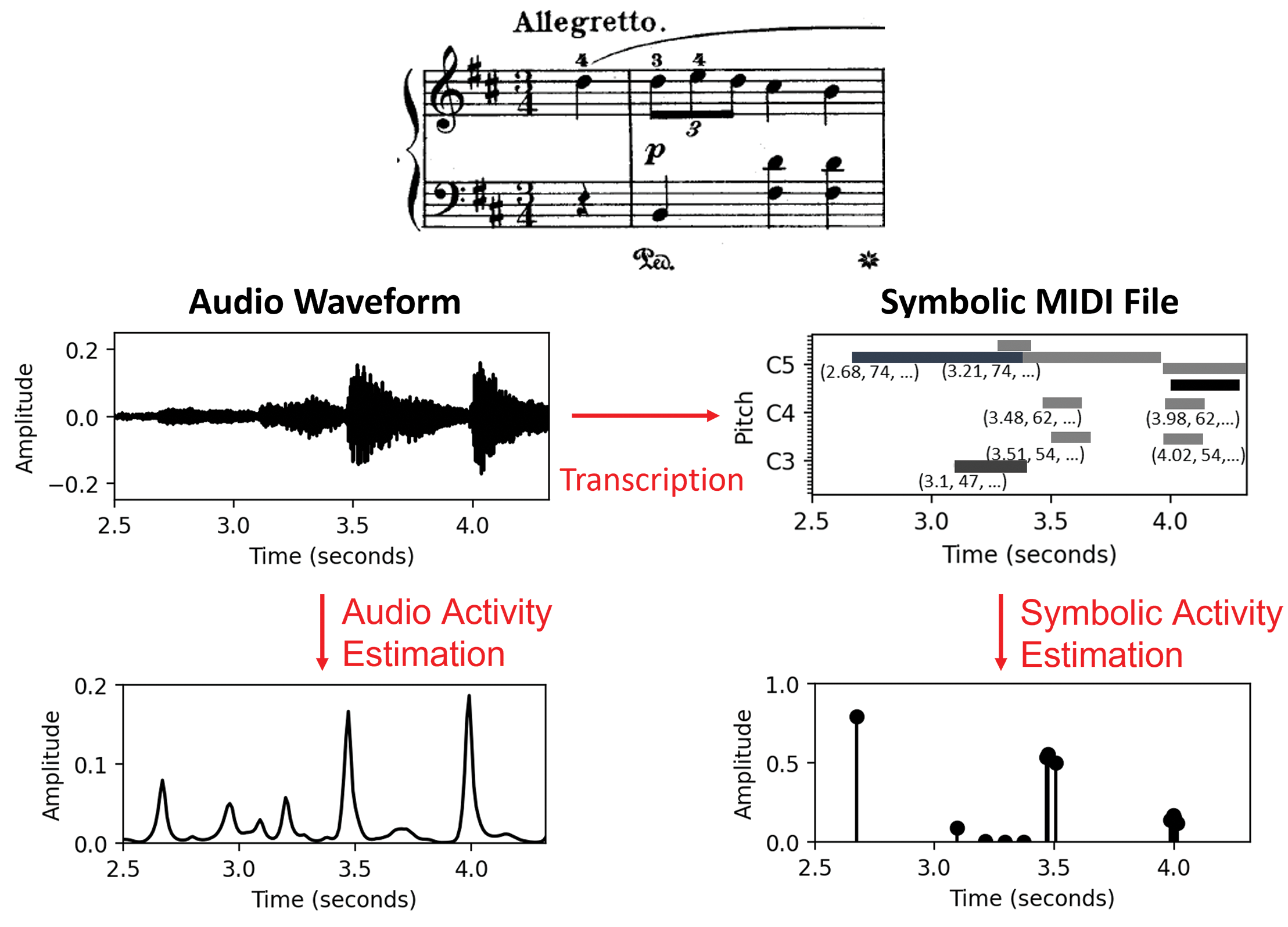
Figure 1
Beat activity estimation of an audio representation using a frame‑based approach (left) and a symbolic representation using an event‑based approach (right).
From a higher‑level viewpoint, beat‑tracking errors can be attributed to both data‑related factors (e.g., musical properties determined by the music scores or physical properties of specific performances (Grosche et al., 2010)) and model‑related factors (e.g., the decision mechanisms of the activity estimators or the assumptions involved in the post‑processors). The choice of evaluation metrics can also bias observations of the model’s true behavior.1 Without systematic control of these factors, the insights we can derive from experiments may be limited. For example, despite the fact that existing works generally report beat‑tracking F1 scores; correct metrical level, with the total of continuous segments (CMLt); and allowed metrical level, with the total of continuous segments (AMLt) (Davies et al., 2009) for various datasets (Chang and Su, 2024; Cheng and Goto, 2023; Hung et al., 2022; Pinto et al., 2021; Zhao et al., 2022), their reliance on the dynamic Bayesian network (DBN) built into madmom (Böck et al., 2016a) or similar approaches (Yamamoto, 2021) imposes strong tempo assumptions, limiting our understanding of what their neural‑network‑based activity estimators truly learn. F1 scores, CMLt, and AMLt also do not allow us to progressively evaluate how well the models handle longer musical contexts. Although researchers have recently recognized the influence of post‑processors and purposely adopted peak‑picking‑based methods (Chiu et al., 2023; Foscarin et al., 2024) without strong assumptions, the impact of peak‑picking thresholds in combination with the overall amplitudes of activation functions has rarely been investigated in detail. Moreover, despite the release and adoption of the Aligned Scores and Performances (ASAP) for the piano transcription dataset (Foscarin et al., 2020), which provides a comprehensive understanding of the limitations of existing deep learning (DL)‑based methods in the context of classical piano music analysis, the musical complexities in the dataset also hinder our understanding of model failures (Chiu et al., 2023; Foscarin et al., 2024).
Considering the issues mentioned above, the goal of this article is to investigate and analyze both symbolic and audio beat trackers, with a better control of factors related to data and models. To the best of our knowledge, the only existing work that compares the two modalities is by Schwarzhuber (2024). However, despite conducting comprehensive experiments regarding network architectures and various input representations, the insights in the work by Schwarzhuber (2024) are also limited by the abovementioned factors: adoption of post‑processors with strong assumptions (i.e., DBN and rule‑based method by Liu et al. (2022)) and limited reported evaluation metrics (i.e., only F1 scores without reporting or discussing precision, recall, or other evaluation metrics). Additionally, there are two types of input data representations used in the beat trackers: spectrograms with evenly distributed time stamps along the time axis (referred to as “frame‑based representation”) and event sequences with unevenly distributed time stamps (referred to as “event‑based representation”). For both representations, there are corresponding post‑processors with very different assumptions, complicating the comparison.
In contrast to existing works, we address the aforementioned factors by establishing a unified post‑processing pipeline to better understand and directly compare the properties of activation functions without altering them significantly, and to derive beat estimations without imposing strong assumptions beyond the mechanisms within the activity estimators. We focus on a cross‑version dataset of five Chopin Mazurkas (Sapp, 2007; 2008) featuring expressive tempo changes (Schreiber et al., 2020; Shi, 2021) and a variety of specified musical properties, including non‑event beats, boundary beats, ornamented beats, constant harmony beats, and weak bass beats that complicate beat tracking (Grosche et al., 2010).2 Furthermore, we propose representation conversion methods combined with various fusion techniques to explore potential ways to leverage the complementarity between audio and symbolic modalities. We start with existing pre‑trained models: madmom (Böck et al., 2016a,b) as a frame‑based audio beat tracker and PM2S (Liu et al., 2022) as an event‑based symbolic beat tracker. More specifically, the madmom activity estimator employs a Bidirectional Long Short‑Term Memory (BiLSTM) network to process audio spectrograms and generate frame‑based activations (as shown in Figure 1, left bottom), while PM2S uses a convolutional recurrent neural network (CRNN) to process MIDI note sequences and generates event‑based activations (as shown in Figure 1, right bottom). We also retrain the BiLSTM and CRNN using the five Mazurkas (Maz‑5) to further investigate the capability of these models to adapt to a specific music scenario and to validate the effectiveness of various late‑fusion methods.
Figure 2 provides a conceptual overview of our cross‑modal approach, featuring two branches: the audio/frame‑based branch (left) and the symbolic/event‑based branch (right). Specifically, in the case of a frame‑based audio beat tracker (Figure 2, left), the audio waveform from a recording is converted to a frame‑based feature representation (e.g., a spectrogram) and processed by an audio activity estimator (purple square) to derive the audio activations . A frame‑based post‑processor (green square) then converts the activations into beat estimations. Similarly, in the case of an event‑based symbolic beat tracker (Figure 2, right), a sequence of event tuples , obtained from a symbolic representation (e.g., a MIDI file), is processed by a symbolic activity estimator (purple square) to derive the corresponding symbolic activations . An event‑based post‑processor (green square) then converts the symbolic activations into beat estimations. In principle, as indicated in Figure 2, one may leverage frame‑to‑event (F2E) and event‑to‑frame (E2F) conversion to bridge the two modalities and explore various fusion methods (blue squares) in both representations, including frame‑based and event‑based fusion.3 In this paper, we focus on the frame‑based representation (left)4 and establish a frame‑based unified post‑processing pipeline (green square) to handle activations from all modalities (i.e., audio, symbolic, and late fusion) consistently, converting them into beat estimations for further analysis.
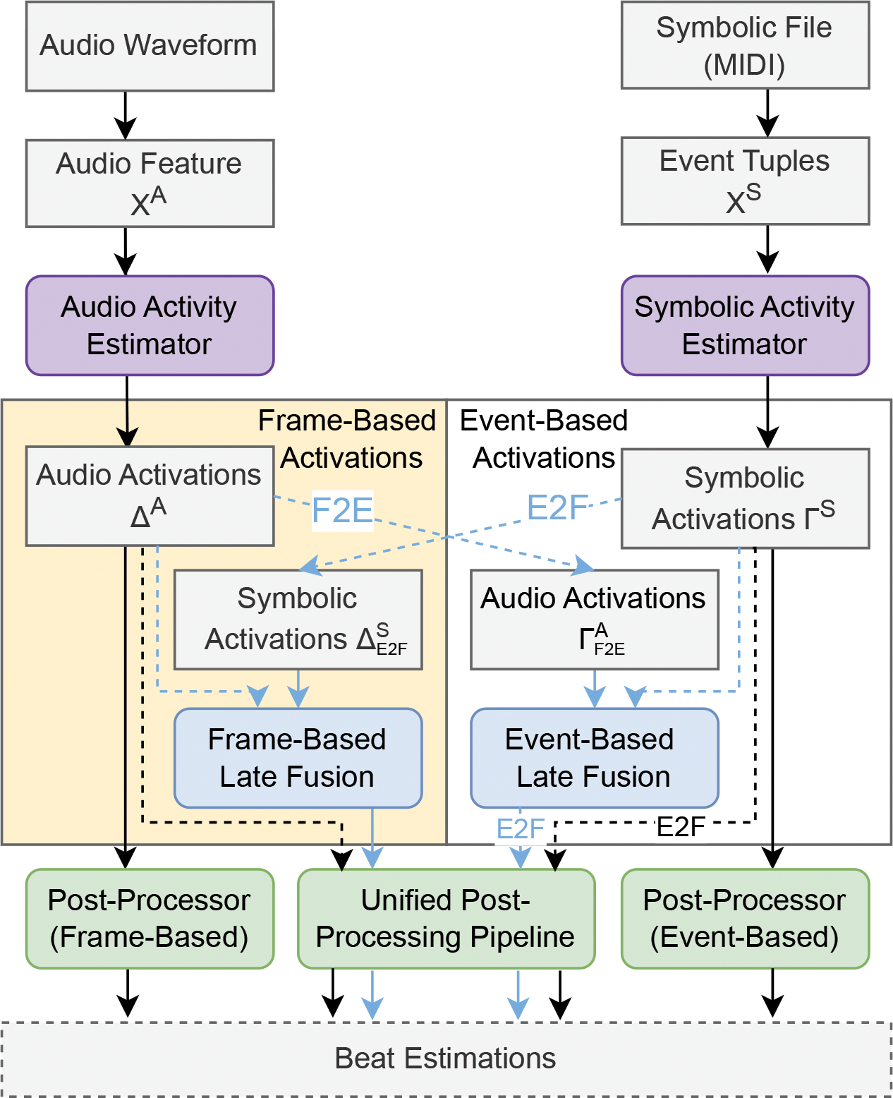
Figure 2
Overview of the system. F2E: frame‑to‑event conversion; E2F: event‑to‑frame conversion.
The remainder of this paper is organized as follows: In Section 2, we introduce the dataset of Chopin Mazurkas (Maz‑5) and our experimental scenarios. In Section 3, we present the mathematical definitions and notations for existing beat‑tracking methods of different modalities. In Section 4, we describe the representation conversion methods. In Section 5, we outline the unified post‑processing pipeline and the peak‑picking method considered. Then, in Section 6, we present the experiment results. In Section 7, we extend the experiment to downbeat tracking and discuss the preliminary results. Finally, we conclude this article in Section 8. We provide the Python source code and supplementary discussions for this paper at GitHub repository: https://github.com/SunnyCYC/CrossModalBeat.
2 Scenario: Chopin Mazurkas
The dataset for our experiments consists of five Chopin Mazurkas (Maz‑5), selected from the Mazurka Project’s collection of 49 Mazurkas.5 For each of the five Mazurkas, Sapp (2007; 2008) manually annotated beat and downbeat positions in 34–88 audio recordings of real performances (Table 1). As a piano dataset featuring expressive tempo changes (e.g., rubato or ritardando), Maz‑5 is typically used for analysis of beat‑tracking errors (Grosche et al., 2010), local tempo (Schreiber et al., 2020), or expressive timing (Shi, 2021). Moreover, the cross‑version scenario (i.e., having multiple recorded performances for each of the Mazurkas) of Maz‑5 allows us to separate musical factors (e.g., musical complexities determined by scores) and physical factors (e.g., audio quality or interpretations of pianists) for beat tracking to gain more insights. Although no performance MIDI files exist for the 301 recordings, recent advances in DL‑based piano transcription enable the creation of MIDI files with sufficient quality for further analysis (e.g., for beat tracking) and to serve as symbolic input representations. For our experiments, we use the transcriber by Kong et al. (2021) to derive MIDI files (without further manual correction). In Section 6, we present the insights gained from these key features of Maz‑5.
Table 1
The five Chopin Mazurkas and their identifiers used in our study. The last three columns indicate the number of beats, performances, and total duration (in hours) available for the respective piece. Dur.: duration; h: hours; ID: identifier; Perf.: performances; Op.: Opus.
| ID | Piece | Number (Beats) | Number (Perf.) | Dur. (h) |
|---|---|---|---|---|
| M17‑4 | Op. 17, No. 4 | 396 | 64 | 4.62 |
| M24‑2 | Op. 24, No. 2 | 360 | 64 | 2.44 |
| M30‑2 | Op. 30, No. 2 | 193 | 34 | 0.80 |
| M63‑3 | Op. 63, No. 3 | 229 | 88 | 3.15 |
| M68‑3 | Op. 68, No. 3 | 181 | 51 | 1.43 |
3 Beat Tracking in Different Modalities
In this section, we present the key concepts, terminology, and mathematical definitions related to audio and symbolic beat‑tracking methods.
3.1 Audio beat trackers
Commonly, an audio beat tracker (ABT) takes as input a spectrogram‑like time–frequency representation (e.g., a Mel spectrogram) calculated from an audio recording and outputs the estimated beat positions. Specifically, an audio beat tracker consists of an audio activity estimator, which processes the input representation and generates an activation function, and a post‑processor, which converts the activation function into beat positions. In this case, the time axis of input data is organized on the basis of regularly sampled frames. From this point forward, we refer to this as the frame‑based organization of the time axis.
In the following, we use the shorthand mathematical formulas based on these two notations: for and . Let denote the frame rate (given in frames per second (FPS)), which specifies the number of frames per second determined by the sampling method. Given a music piece with a duration of seconds, we assume that the (spectrogram‑like) audio feature representation is provided by a matrix encoded as follows:
where denotes the total number of frames and represents the number of features. An audio beat activity estimator takes as input and generates the following activation function:
which maps each time frame to its corresponding likelihood (or pseudo‑probability) of being a beat. See Figure 3a for an example of . A frame‑based post‑processor can then analyze the activation function and determine the estimated beats (as frame indices) . Here, is a sequence of length consisting of strictly monotonically increasing beat positions for . Common frame‑based post‑processors include predominant local pulse (PLP) (Grosche and Müller, 2011; Meier et al., 2024), dynamic programming‑based approaches (Ellis, 2007) such as dynamic Bayesian networks (DBNs) (Böck et al., 2016b), and conditional random field‑based methods (CRFs) (Fuentes et al., 2019).
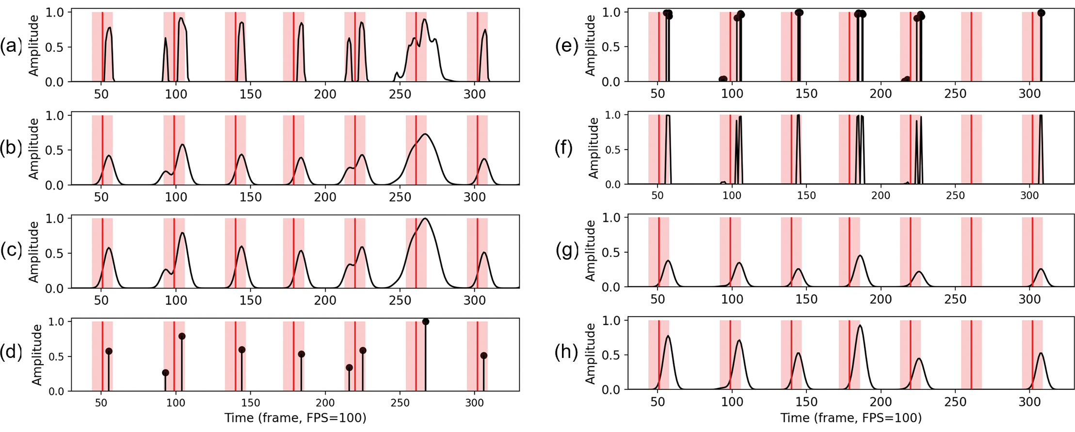
Figure 3
Processing of beat activation functions. (a) Frame‑based activation function from an audio activity estimator. (b) Gaussian smoothing of (a). (c) Max normalization of (b). (d) Peak‑picking results of (c). (e) Event‑based activation function from a symbolic activity estimator. (f) Event‑to‑frame conversion of (e). (g) Gaussian smoothing of (f). (h) Max normalization of (g). Red vertical lines indicate reference annotated beats. Red regions highlight the 70 ms tolerance window.
3.2 Symbolic beat trackers
For a symbolic beat tracker (SBT) that consists of a symbolic activity estimator and a post‑processor, the symbolic input can be organized in either a frame‑based manner (as introduced in Section 3.1) using piano‑roll‑like input representations (Chuang and Su, 2020), or using an event‑based representation (e.g., an event sequence). In this study, we focus on PM2S,6 which takes as input an event sequence obtained from MIDI files (Liu et al., 2022) and generates an event‑based activation function. Specifically, for an event‑based method, the time axis of input data is organized on the basis of a list of unevenly distributed time stamps. These time stamps could be the timing of any musical attributes encoded by a set , such as pitches, durations, note velocity, instrumentation, or others (Liu et al., 2022). For instance, in the context of MIDI, may represent the set of possible MIDI pitch and velocity values for a note. Given a list of time stamps (in seconds) noted as , with and , the input representation of an event‑based symbolic activity estimator can be organized as a list
where attribute , and . A tuple is also called an event.
An event‑based symbolic activity estimator takes as input and generates as output the following activation function:
Specifically, the event‑based symbolic activation function maps a time index to a tuple with a time stamp and a pseudo‑probability for that time position to be a beat. See Figure 3e for an example of .
An event‑based post‑processor (Liu et al., 2022) can analyze the event‑based activation function and generate estimated beat positions , where is a sequence of length consisting of strictly monotonically increasing beat positions with for .
4 Event‑to‑Frame Activation Conversion
In this section, we describe our approach to event‑to‑frame (E2F) conversion, which not only allowd us to bridge the frame‑based audio and the event‑based symbolic activations for further fusion but also enables us to process activations from all modalities consistently for subsequent analysis.
Given a list of monotonically increasing time points with and the corresponding event‑based activation function , with , we can convert it into a frame‑based representation based on a specified frame rate . Let with be the total number of frames, then we define
for . Note that is the frame index corresponding to the time stamp . To account for the case where several time stamps are assigned to the same frame index, we further define
to keep the maximum probability among those stamps. The converted event‑based activation function is then defined as follows:
for . Figure 3e and 3f provides an example of E2F conversion.
5 Unified Post‑Processing Pipeline
As mentioned in Section 1, we establish a unified post‑processing pipeline to handle activations of all modalities (i.e., audio, symbolic, and fused) consistently, aiming to preserve the original properties of the activations without imposing strong assumptions. This is mainly achieved by converting all event‑based activations to frame‑based activations using E2F conversion, smoothing and normalizing all derived frame‑based activations, and then applying peak‑picking with explicit and transparent settings. In this section, we describe our methods for smoothing and normalizing (Section 5.1), and peak‑picking methods with three types of threshold settings (Section 5.2 and Section 5.3). The effectiveness of these methods are then justified in Section 6.2.
5.1 Smoothing and normalization
As pointed out by Müller and Chiu (2024), novelty enhancement strategies, such as smoothing and normalization, are essential before peak‑picking. By applying Gaussian smoothing and max normalization, we can reduce spurious peaks caused by irrelevant fluctuations, filter out peaks occurring at a frequency too high for natural beat tracking, and standardize the activation values to make them comparable and treatable as pseudo‑probabilities.
For each frame‑based activation function, following Müller and Chiu (2024), we first apply a one‑dimensional Gaussian filter, defined in Equation (8), to smooth out irrelevant local fluctuations. Let
be a truncated Gaussian function, where . Taking into account the conventional tolerance window of ms for beat‑tracking evaluation, we empirically fixed (frames) at a frame rate of FPS. After smoothing, we apply max normalization7 by dividing each activation function by its maximum value to scale all values to the range . Figure 3 illustrates the effects of Gaussian smoothing and max normalization.
5.2 Global threshold
One of the simplest methods to convert activation functions into estimated beat positions is to apply peak‑picking with a global fixed threshold , e.g., . Despite being simple and commonly adopted (Böck et al., 2016b; Chiu et al., 2023; Foscarin et al., 2024), this method is sensitive to the threshold values. While a high threshold may remove too much information from the activation functions and lead to a low recall value, a low threshold may retain noise or irrelevant activation peaks, and lead to a low precision value. The optimal threshold for each track depends on both the data and the model (i.e., activity estimator) and is generally unknown or not specified in many use cases. In this study, we experiment with thresholds .
Additionally, given the reference annotated beat positions, one can also investigate the upper bound performance of an activation function by performing a grid search. Specifically, a range of global peak thresholds (i.e., ) is defined, and peak‑picking is applied with each threshold to each test track, reporting only the highest F1 scores. We refer to this reference‑informed method as “oracle threshold.”
5.3 Adaptive local threshold
In contrast to a fixed global threshold, an adaptive threshold that adjusts on the basis of the local properties of the activation function is generally more robust and less sensitive to the hyperparameter settings (Müller and Chiu, 2024). In this study, we determine a local average function defined by
and use it as the local threshold of the peak‑picking. The and the parameter sets the size of the averaging window. Zero padding is applied to avoid summation over negative indices. In this study, we experiment with corresponding to 5, 10, or 20 seconds.
6 Experiments
In this section, we first describe the evaluation metrics (Section 6.1), then report our experiment results of pretrained models (Section 6.2) and retrained models (Section 6.3), followed by a discussion of insights derived from the Maz‑5 scenario (Section 6.4).
6.1 Evaluation metrics
Following the conventional evaluation setting for beat tracking, we adopt from mir_eval the metrics of F1 score (F1), precision (P), and recall (R) with an error tolerance of ms. Furthermore, we also compute the L‑correct metric (Chiu et al., 2022; Grosche and Müller, 2011) to evaluate how well the beat trackers can handle a longer musical context. Rather than evaluating each annotated reference beat individually, the L‑correct metric requires that at least consecutive reference beats are correctly detected, where is an adjustable parameter. In this work, we report the F‑measure of L‑correct with , denoted as F‑L*.
6.2 Pretrained beat trackers
In this section, we evaluate the pretrained activity estimators (i.e., madmom for audio modality and PM2S for the symbolic one) using our unified post‑processing pipeline (Section 5) and the Maz‑5 dataset. Since neither of these two systems was trained on the Maz‑5 dataset, the evaluation fairly and accurately reflects their performance on unseen classical music. We also experiment with late fusion of the two modalities to investigate the underlying complementarity between the two types of models.
6.2.1 Activity estimators and post‑processors
Both madmom and PM2S can jointly generate beat and downbeat activations. In this work, we focus more on the beat activations. For the audio modality () we adopt the RNNDownBeatProcessor of madmom to derive the beat activations . For the symbolic modality (), we first transcribe the 301 recordings using the model by Kong et al. (2021) to derive MIDI files. We then apply the CRNN activity estimator by Liu et al. (2022) (referred to as PM2S) to derive the beat activation functions . Finally, we conduct the E2F conversion to derive . As described in Section 5, these frame‑based activation functions will be smoothed and normalized before peak‑picking. We further experiment with two simple late‑fusion methods: addition‑based () and (element‑wise) multiplication‑based () methods. Specifically, we take the smoothed and normalized activation functions of single modalities (i.e., and ), add them up or multiply them point‑wise, and smooth and normalize the fused activations again before peak‑picking.
As described in Section 5, for all the derived frame‑based activations mentioned above, we apply peak‑picking with three types of threshold settings, including a global (GLB) threshold, an adaptive local (LOC) threshold, and an oracle threshold, respectively.
6.2.2 Effects of peak‑picking thresholds
Table 2 presents the beat‑tracking results of pretrained single‑modality models (ABTs and SBTs) derived using three types of peak‑picking settings (GLB, LOC, and oracle).8 We specify the hyperparameters using a dash symbol; for example, GLB‑0.1 indicates a global threshold with , and LOC‑20 indicates a local threshold using a window length of 20 seconds. The following observations can be made: Under the GLB threshold setting, the performances of ABTs and SBTs across all evaluation metrics show high sensitivity to the threshold values. For example, increasing the global threshold from 0.25 to 0.5 reduces the F1 score for ABTs from 0.886 to 0.660 (−0.226) and for SBTs from 0.775 to 0.662 (−0.113). Using the oracle threshold setting reveals upper bound F1 scores for ABT (0.892) and SBT (0.855). Under the LOC threshold setting, while the achieved F1 scores may be slightly below the GLB best case (e.g., for ABT, GLB‑0.25: 0.886 vs. LOC‑5: 0.835), they remain comparable and exhibit substantially lower sensitivity to hyperparameter settings. Specifically, varying the window length of LOC threshold setting has only a small impact across all evaluation metrics.
Table 2
Work‑wise average beat‑tracking results for pretrained models. (Top) madmom‑based audio beat trackers. (Bottom) PM2S‑based symbolic beat trackers. The best results are highlighted in bold. GLB: global; LOC: local.
| Threshold | F‑measure | L‑correct | ||||
|---|---|---|---|---|---|---|
| F1 | P | R | F‑L2 | F‑L3 | F‑L4 | |
| Audio beat trackers (ABTs) | ||||||
| GLB‑0.01 | 0.7570.054 | 0.6320.071 | 0.9680.020 | 0.5490.116 | 0.4760.130 | 0.4090.140 |
| GLB‑0.1 | 0.8250.053 | 0.7300.074 | 0.9630.021 | 0.6980.101 | 0.6390.119 | 0.5650.140 |
| GLB‑0.25 | 0.8860.048 | 0.8770.056 | 0.9010.053 | 0.8310.080 | 0.7950.098 | 0.7460.125 |
| GLB‑0.5 | 0.6600.108 | 0.9550.037 | 0.5180.118 | 0.4870.160 | 0.3720.174 | 0.2840.161 |
| Oracle | 0.8920.045 | 0.8660.061 | 0.9230.044 | 0.8420.071 | 0.8090.089 | 0.7590.120 |
| LOC‑5 | 0.8350.047 | 0.7480.066 | 0.9580.024 | 0.7450.080 | 0.6960.098 | 0.6280.121 |
| LOC‑10 | 0.8400.048 | 0.7550.067 | 0.9580.024 | 0.7460.082 | 0.6960.100 | 0.6270.124 |
| LOC‑20 | 0.8380.048 | 0.7510.068 | 0.9600.024 | 0.7370.084 | 0.6860.102 | 0.6160.125 |
| Symbolic beat trackers (SBTs) | ||||||
| GLB‑0.01 | 0.8230.045 | 0.7410.064 | 0.9370.038 | 0.7000.092 | 0.6060.123 | 0.4970.148 |
| GLB‑0.1 | 0.8360.056 | 0.8770.064 | 0.8040.072 | 0.7230.101 | 0.6480.129 | 0.5680.149 |
| GLB‑0.25 | 0.7750.070 | 0.9130.057 | 0.6790.091 | 0.5890.135 | 0.4880.161 | 0.4000.175 |
| GLB‑0.5 | 0.6620.092 | 0.9350.052 | 0.5220.107 | 0.3710.163 | 0.2580.174 | 0.2010.168 |
| Oracle | 0.8550.048 | 0.8450.072 | 0.8700.052 | 0.7670.084 | 0.6980.114 | 0.6210.138 |
| LOC‑5 | 0.8410.056 | 0.9150.055 | 0.7820.069 | 0.7450.100 | 0.6760.131 | 0.6020.152 |
| LOC‑10 | 0.8420.056 | 0.9150.055 | 0.7830.068 | 0.7460.099 | 0.6770.129 | 0.6040.152 |
| LOC‑20 | 0.8440.055 | 0.9150.055 | 0.7860.067 | 0.7500.097 | 0.6820.128 | 0.6100.150 |
Moreover, as mentioned in Section 5.2, selecting an optimal global threshold involves a precision–recall trade‑off that can obscure the models’ original behaviors. For instance, adjusting the global threshold from 0.01 to 0.5 raises ABT precision from 0.632 to 0.955 (+0.333) but decreases recall from 0.968 to 0.518 (−0.450). Opposed to GLB, the LOC method determines the threshold on the basis of the average amplitude within each window, thus compensating for local changes in intensity or dynamics. Under this LOC setting, differences between ABTs and SBTs become more apparent: ABTs tend to achieve higher recall, while SBTs generally attain higher precision, highlighting the potential complementarity between the two methods based on different modalities and concepts. Lastly, the adaptation capability of LOC also stabilizes the L‑correct results. When increases from 2 to 4, the GLB‑based methods often show a dramatic drop in F1 scores. For example, for SBT, GLB‑0.01 decreases from 0.700 to 0.497 (−0.203) and GLB‑0.1 decreases from 0.723 to 0.568 (−0.155), while LOC‑20 shows a slightly smaller decrease, from 0.750 to 0.610 (−0.140). This may be because expressive music often demonstrates dramatic musical changes (e.g., in volume or tempo), which fail the global settings (since any single error can break the continuity of L‑correct). However, these dramatic changes may remain locally consistent, allowing adaptive methods to partially capture them.
In summary, we can see that, despite being simple and free from strong assumptions, the use of GLB still requires a careful selection of the threshold, which could potentially obscure the properties of activation functions. We therefore suggest LOC as a neutral post‑processor to better reflect the behavior of the activation functions.
6.2.3 Effects of late fusion
With the overall good performance using LOC and its stability across the hyperparameter , we now fix the peak‑picking setting to LOC with a window length of 20 seconds (LOC‑20) and investigate the behavioral differences between single‑modality beat trackers and late fusion‑based models. Table 3 (top) presents the work‑wise average beat‑tracking results for audio recordings of Maz‑5. From the F1 scores, we can observe improvements made by both addition‑based () and multiplication‑based () methods. For example, the F1 score increases from 0.844 for to 0.885 for and to 0.850 for . Specifically, and represent two ways to leverage the complementarity between and : recall‑oriented and precision‑oriented, respectively. While retains only the activation peaks agreed upon by both and , leading to much higher precision than and (: 0.959; : 0.751; : 0.915), retains all strong activation peaks from either or , leading to a high recall (: 0.947; : 0.960; : 0.786).
Table 3
Work‑wise average of beat‑tracking results (including late‑fusion approaches). Beat‑tracking results (including late‑fusion approaches) were derived using peak‑picking with local average threshold with a window length of 20 seconds (LOC‑20). The best results are highlighted in bold.
| Activation | F‑measure | L‑correct | ||||
|---|---|---|---|---|---|---|
| F1 | P | R | F‑L2 | F‑L3 | F‑L4 | |
| Pretrained | ||||||
| 0.8380.048 | 0.7510.068 | 0.9600.024 | 0.7370.084 | 0.6860.102 | 0.6160.125 | |
| 0.8440.055 | 0.9150.055 | 0.7860.067 | 0.7500.097 | 0.6820.128 | 0.6100.150 | |
| 0.8850.044 | 0.8380.063 | 0.9470.027 | 0.8230.071 | 0.7900.086 | 0.7440.109 | |
| 0.8500.051 | 0.9590.035 | 0.7650.067 | 0.7490.093 | 0.6840.121 | 0.6100.142 | |
| Retrained | ||||||
| 0.8160.038 | 0.7160.054 | 0.9650.014 | 0.6960.068 | 0.6060.087 | 0.4680.100 | |
| 0.9270.037 | 0.9190.042 | 0.9380.037 | 0.9020.053 | 0.8820.066 | 0.8580.082 | |
| 0.8600.036 | 0.7860.054 | 0.9620.015 | 0.7720.064 | 0.7120.079 | 0.6250.107 | |
| 0.9370.034 | 0.9430.031 | 0.9330.041 | 0.9170.047 | 0.8990.059 | 0.8820.069 | |
Figure 4 (left) visualizes the behaviors of all these pretrained models. Comparing the musical score as a reference, we can observe the different behaviors between the four methods: When there are multiple note onsets close together (e.g., around the frame 4700 and the frame 4800, between the last beat of measure 40 and the second beat of measure 41 in the score), and generate different peaks in the activation function that do not correspond to the annotations. As these non‑beat peaks are weak, the addition, smoothing, and normalization process of addition‑based fusion can remove them, improving the performance of . On the other hand, eliminates the non‑beat peaks around frame 4700 via the multiplication process. Figure 4 (left) also explains why the L‑correct scores can be largely improved for in Table 3: While will fail if either or makes a false‑negative prediction, breaking the continuity required by L‑correct, will retain strong activation peaks from either or while smoothing out weak predictions.
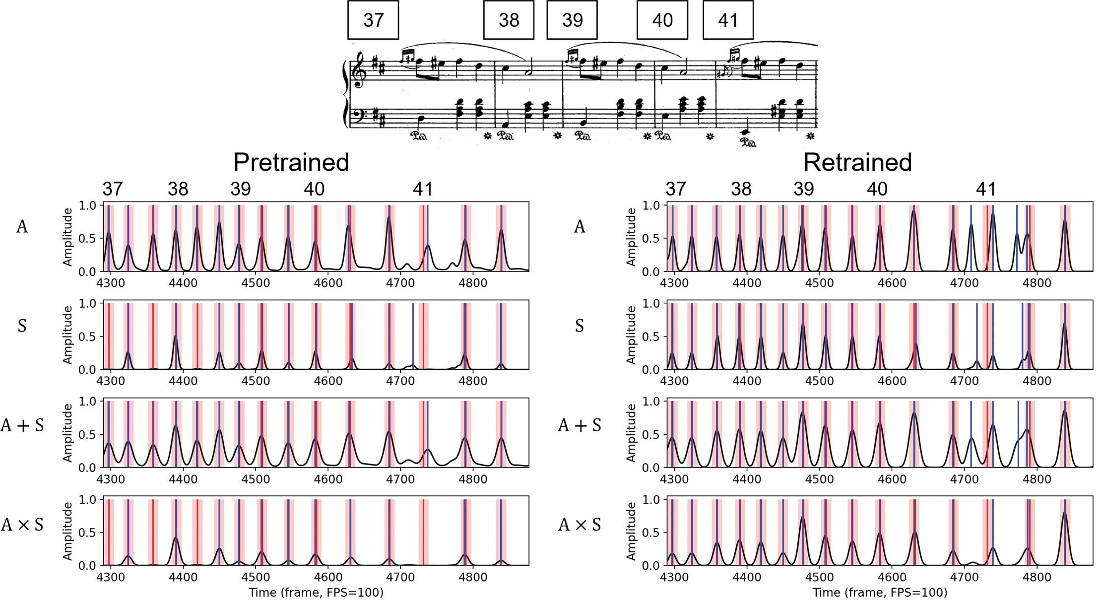
Figure 4
Comparison of four types of activations. (top) Music score of Op. 30, No.2. (left) Activation functions from pretrained models. (right) Activation functions from retrained models. Red regions highlight the 70 ms tolerance window. Blue vertical lines indicate the beat estimations derived using peak‑picking with the LOC‑20 threshold setting. Op.: Opus.
6.3 Retrained beat trackers
The pretrained models were trained on datasets independent of Maz‑5; for example, the madmom BiLSTM was primarily trained on pop, rock, and dance music, while the PM2S CRNN was trained on classical piano music by various composers, excluding Maz‑5. In the next experiment, we retrained the same models (i.e., BiLSTM and CRNN) from scratch using Maz‑5 with five‑fold cross‑validation. This approach not only enables model evaluation with limited data but also ensures that all performances (versions) in the Maz‑5 dataset appear at least once in both the training and test sets. Specifically, we split the five Mazurkas into five folds. For each split, three Mazurkas are used for training, one for validation, and one for testing. In general, retraining allows us to inspect the capability of a model to adapt to a specific music scenario (e.g., Chopin Mazurkas). In this section, we describe our retraining methods, conduct experiments similar to those for the pretrained models, and discuss the consistencies and differences between the pretrained and retrained results.
6.3.1 Activity estimators and post‑processors
Taking the retrained single‑modality models, we apply them to the corresponding test split to derive the activations. We then apply similar late‑fusion method and unified post‑processing (as those used for the pretrained models) to the activations to derive beat estimations for further analysis.
6.3.2 Effects of peak‑picking thresholds
Figure 5 visualizes and summarizes the observed effects of peak‑picking thresholds. Despite that fact that both pretrained (Figure 5a) and retrained (Figure 5b) models show a strong dependency on GLB threshold values (solid curves), this dependency is less pronounced for the retrained models, particularly for small thresholds. Furthermore, compared with the pretrained models, the retrained models show an overall improvement in F1 scores, along with shifts in optimal global thresholds (e.g., pretrained : 0.0625; retrained : 0.125). This again highlights the challenge of identifying the optimal global threshold in practical applications. However, the local threshold‑based results (dashed lines), though not the best, generally perform close to the best case of GLB settings.
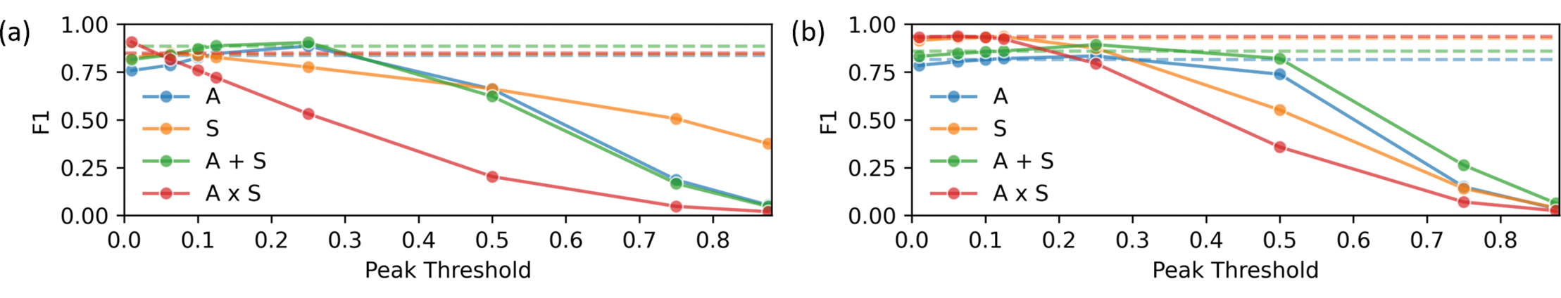
Figure 5
Effects of peak‑picking thresholds on beat‑tracking F1 scores. (a) Pretrained models. (b) Retrained models. Dashed lines indicate the F1 scores of the corresponding results derived using local average threshold (LOC‑20). Solid dots indicate the F1 scores derived using global threshold values .
6.3.3 Effects of training data
Going beyond Figure 5, Table 3 reveals further differences between pretrained (top) and retrained (bottom) models. While the retrained ABT behaves similarly to a pretrained ABT (retrained F1: 0.816; pretrained F1: 0.838), the retrained SBT achieves much higher scores for all metrics compared with the pretrained SBT (e.g., retrained F1: 0.927; pretrained F1: 0.844), indicating that the event‑based CRNN model may have higher capability to learn (or, in some way, overfit to) the musical patterns in Maz‑5. Figure 4 illustrates the differences between the pretrained (left) and retrained (right) models. For audio activations (), both pretrained and retrained BiLSTMs show a tendency to detect onsets and generate activation peaks at non‑beat positions (e.g., between frames 4700 and 4800). However, the retrained BiLSTM produces sharper, higher peaks, suggesting greater sensitivity to Maz‑5 note events. For symbolic activations, both pretrained and retrained CRNNs produce less pronounced activation peaks compared with the BiLSTMs (e.g., around frames 4700–4800), yet the retrained CRNN appears to capture different musical patterns and retains more accurate peaks than the pretrained version (e.g., around frames 4350–4450).
6.3.4 Effects of late fusion
The improvement in retrained SBT noted above also influences the effects of late‑fusion methods. In Table 3 (bottom), we see that addition‑based fusion () no longer outperforms SBT (), whereas multiplication‑based fusion () still does. This shift is primarily due to two factors. First, the recall of retrained increases significantly, from 0.786 to 0.938, which also substantially boosts the recall of retrained (from 0.765 to 0.933). Second, the retrained appears more sensitive to Maz‑5 note events, generating stronger peaks at non‑beat positions, which reduces its precision (from 0.751 to 0.716) and, in turn, lowers the precision of retrained as well. Additionally, late‑fusion methods prove to be less effective than in the pretrained case. Specifically, as retrained becomes much stronger and retrained slightly weaker, the reduced complementarity between the two modalities limits the benefits of fusion. In summary, similar to our findings regarding optimal global threshold, the optimal fusion method is also dependent on the model and the data, which are mostly unknown for real use cases. This raises the question of whether DL‑based methods can learn a more effective approach to fusing the two modalities based on the provided musical content, which is beyond the scope of this article.9
6.4 Insights from Maz‑5 scenario
We further color‑code the F1 scores of Maz‑5, as shown in Figure 6. One can observe that the effectiveness of all models is version‑dependent; i.e., they depend on the properties of specific versions. For example, versions #31, #40, #50, and #71 of M63‑3 are consistently more challenging for all models compared with other versions. A possible explanation is the poor audio quality of the recordings and the varied interpretations by pianists (e.g., left‑hand onsets may intentionally not align with right‑hand onsets). Despite the version dependency, one can still observe certain trends of the average (right side after the black vertical line). Consistent with our observations in Table 3, for the pretrained cases, typically works better than and . Interestingly, in the retrained case, the improvement of becomes more evident in the color‑coded plot, shown as a horizontal blue line (for M63‑3) that contrasts with the original results. Aside from cases of poor audio quality (e.g., version #50), which introduce errors during transcription, retrained appears to adapt well to the Maz‑5 scenario and to overcome certain version‑wise challenges (e.g., for M63‑3, retrained performs well on versions #35, #36, and #71–73, which are challenging for all pretrained models). Lastly, one can also observe the challenges posed by musical properties by comparing across the five Mazurkas. For example, M24‑2 and M30‑2 are noticeably easier for all models. This is partly because the number of non‑beat note events is lower in these Mazurkas. In summary, the cross‑version nature of the Maz‑5 scenario, combined with the color‑coded plot, not only aligns with our previous observations but also offers deeper insights into version dependency, adaptation to specific music scenarios, and model limitations (e.g., challenges in handling low‑quality recordings).
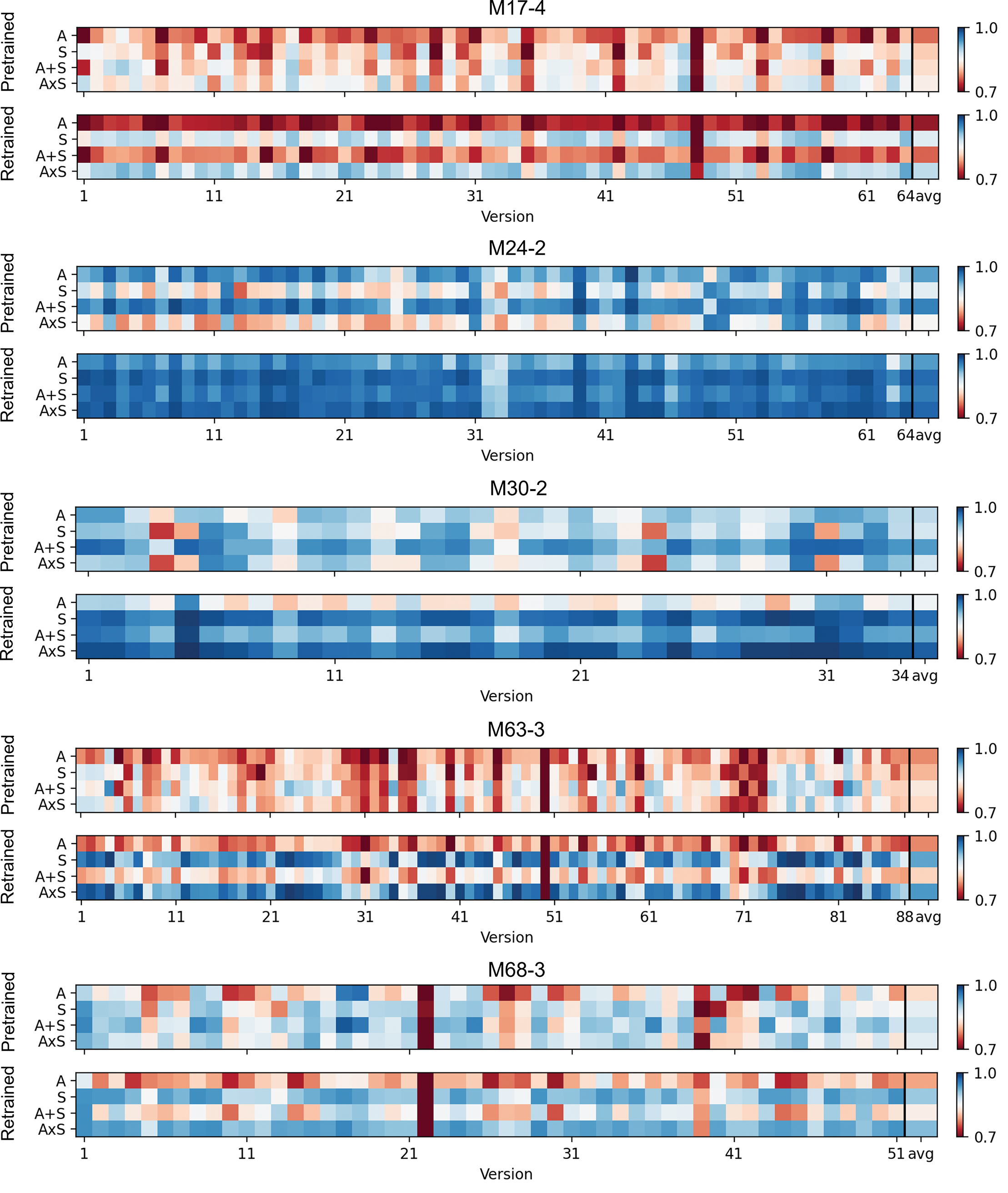
Figure 6
Beat‑tracking F1 scores of Maz‑5.
7 Toward Downbeat Tracking
We now repeat the experiments for downbeat tracking to assess whether the insights gained from beat tracking extend to downbeats, which rely on higher‑level metrical structures rather than just local onset information. While beat tracking primarily detects rhythmic pulses, downbeat tracking requires understanding phrase structures, harmonic cues, and long‑term dependencies, making it a substantially more difficult task. Rather than aiming to improve downbeat estimation, this experiment explores the potential of fusing different modalities for this challenging problem.
Using the same experimental pipeline, we evaluate downbeat activations from pretrained and retrained audio beat trackers () and symbolic beat trackers (), as well as their fusion variants ( and ). As shown in Table 4, the pretrained models perform poorly in downbeat tracking, with all F1 scores below 0.500 and L‑correct measures under 0.100, indicating low quality in capturing the continuity of downbeat estimations. While the pretrained model maintains high recall (0.897), the pretrained model does not retain its precision advantage from beat tracking (0.309 vs. 0.915 in Table 3), suggesting that downbeat tracking is a task that is more complex for and less effectively learned by these models. Given these limitations, late fusion provides little improvement.
Table 4
Work‑wise average of downbeat‑tracking results (including late‑fusion approaches). Downbeat‑tracking results (including late‑fusion approaches) were derived using peak‑picking with local average threshold with a window length of 20 seconds (LOC‑20). The best results are highlighted in bold.
| Activation | F‑measure | L‑correct | ||||
|---|---|---|---|---|---|---|
| F1 | P | R | F‑L2 | F‑L3 | F‑L4 | |
| Pretrained | ||||||
| 0.4500.039 | 0.3010.030 | 0.8970.061 | 0.0190.013 | 0.0080.005 | 0.0070.002 | |
| 0.4350.049 | 0.3090.036 | 0.7440.093 | 0.0270.021 | 0.0130.014 | 0.0100.010 | |
| 0.4590.040 | 0.3120.029 | 0.8760.069 | 0.0190.012 | 0.0080.006 | 0.0070.002 | |
| 0.4480.064 | 0.3470.050 | 0.6400.105 | 0.0840.047 | 0.0320.028 | 0.0180.019 | |
| Retrained | ||||||
| 0.4010.026 | 0.2540.020 | 0.9610.029 | 0.0100.004 | 0.0050.001 | 0.0050.001 | |
| 0.6570.071 | 0.5610.072 | 0.8140.080 | 0.4800.100 | 0.4320.102 | 0.3960.101 | |
| 0.4340.026 | 0.2810.021 | 0.9710.025 | 0.0160.007 | 0.0080.004 | 0.0070.003 | |
| 0.6710.073 | 0.5910.072 | 0.7910.082 | 0.5190.103 | 0.4710.109 | 0.4330.111 | |
Retraining the models follows a similar trend as in beat tracking. The retrained model exhibits greater sensitivity to note events in Maz‑5, improving recall (from 0.897 to 0.961) but at the cost of reduced precision (from 0.301 to 0.254). The retrained model shows substantial improvements in both precision (from 0.309 to 0.561) and recall (from 0.744 to 0.814), significantly boosting L‑correct scores (from below 0.100 to above 0.390). As in beat tracking, the precision‑oriented fusion method () further enhances the F1 score (from 0.657 to 0.671) by slightly lowering recall (from 0.814 to 0.791) while improving precision (from 0.561 to 0.591).
Overall, late fusion is beneficial only when both modalities provide meaningful and complementary outputs. The strong improvements in retrained for both tasks suggest that event‑based representations with explicitly defined note events offer a more effective approach for classical music, capturing musical structure and phrasing more effectively than audio‑based methods alone.
8 Conclusion
In this work, we developed a cross‑modal approach to beat tracking, aiming to deepen our understanding of audio and symbolic beat trackers while exploring their complementarity through fusion methods. Using a dataset of Chopin Mazurkas (Maz‑5), we evaluated pretrained models in a controlled musical scenario and introduced a unified post‑processing pipeline to enable direct comparisons, mitigating confounding effects from conventional post‑processors. Retraining the models provided insights into their adaptability to Maz‑5, revealing that symbolic‑based methods benefit more from domain‑specific training. Our exploration of late‑fusion strategies demonstrated how combining audio and symbolic modalities can enhance performance by balancing precision and recall. To extend our analysis, we also investigated downbeat tracking to assess whether insights from beat tracking generalize to this more complex task. While retraining and fusion exhibited similar trends in both beat and downbeat tracking, the overall performance metrics were notably lower in the latter, highlighting the additional challenges of downbeat tracking. Beyond these findings, our work provides a structured framework for analyzing beat tracking across different input modalities. Future research could further refine fusion strategies and explore broader datasets to enhance the robustness of rhythm analysis techniques.
Funding Information
This work was funded by the Deutsche Forschungsgemeinschaft (DFG;, German Research Foundation) within the project “Learning with Music Signals: Technology Meets Education” under Grant No. 500643750 (MU 2686/15‑1) and the Emmy Noether research group “Computational Analysis of Music Audio Recordings: A Cross‑Version Approach” under No. 531250483 (WE 6611/3‑1). The International Audio Laboratories Erlangen are a joint institution of the Friedrich‑Alexander‑Universität Erlangen‑Nürnberg (FAU) and Fraunhofer Institute for Integrated Circuits IIS.
Competing Interests
The authors have no competing interests to declare.
Author Contribution
Ching‑Yu Chiu was the primary contributor and lead author of this article. Ching‑Yu Chiu and Lele Liu jointly implemented the fusion approach and conducted the experiments. Meinard Müller and Christof Weiß supervised the work and contributed to the writing. All authors were actively involved in developing the conceptual framework and preparing the final manuscript.
Notes
[1] In general, every evaluation metric has its limitations and provides insights from specific perspectives. While the F‑measure is simple and concise, it does not reflect a model’s ability to make continuous correct estimations (Davies et al., 2021; 2009). CMLt and AMLt (Davies et al., 2009), designed to evaluate models in a continuity‑based manner, require at least two consecutive correct estimations. In contrast, L‑correct (Grosche and Müller, 2011) allows for manual adjustment of the continuity length criterion. Moreover, these metrics do not account for metric‑level switching behaviors in beat‑tracking models. For a more detailed discussion of the potential inconsistencies and limitations of existing metrics, readers can refer to Chiu et al. (2022).
[2] While the use of a single dataset indeed limits the generalizability of this study, analyzing additional datasets would introduce considerable complexities (e.g., changes in time signatures or underlying inconsistencies between musical styles that may influence model learning), requiring discussion beyond the scope of this work. As our goal is to understand existing models in a carefully controlled setting rather than propose an approach aimed at significant performance improvements, we focus on Maz‑5 in this study.
[3] Given the space limitations and the relatively limited insights gained, we omit the event‑based late‑fusion experiments in this paper and report the results in our GitHub repository: https://github.com/SunnyCYC/CrossModalBeat.
[4] The conversion from a frame‑based to an event‑based representation involves more technical decisions and may result in greater information loss. Therefore, we adhere to the frame‑based representation, as it is more fundamental.
[5] The Mazurka Project: http://www.mazurka.org.uk, 2010
[6] In Liu et al. (2022), the model is referred to as Performance MIDI‑to‑Score (PM2S), which consists of both an activity estimator and a rule‑based post‑processor. In this work, we use only the activity estimator and refer to it as PM2S.
[7] Note that there are more advanced local maxima‑based normalization methods to further improve the tracking performance of the activation function (Nunes et al., 2015). However, as our goal is to understand rather than to improve the activation function, we consciously avoid complicated processing methods or fine‑tuning of the processing parameters.
[8] In this article, we omit the results and discussions of conventional post‑processors such as DBN (Böck et al., 2016a; Krebs et al., 2015) and DP (Ellis, 2007; McFee et al., 2015) owing to the confounding effects introduced by their strong tempo assumptions and their poor performance (all F1 scores below 0.750; see our GitHub repository for details). For a detailed discussion on the failure of DBN and DP on the Maz‑5 dataset and how they may hinder the properties of the activation functions, readers may refer to Chiu et al. (2023).
[9] Preliminary results of training‑based fusion can be found in our GitHub repository: https://github.com/SunnyCYC/CrossModalBeat.