
1 Introduction
Meter tracking, in particular beat and downbeat tracking, is a fundamental task in music information retrieval (MIR). It is concerned with the automatic estimation of temporal regularities in music, on many hierarchical levels (beats, measures, hypermeasures, etc.). At the surface, it corresponds to determining groups of perceived pulse positions, with the main pulse (tactus) generally being identified as the beat, i.e., the points in time where a human would tap while listening to music. It is worth noting that beat perception can be influenced by a subject’s musical training and cultural background (Misgeld et al., 2021). Many applications rely heavily on the accurate extraction of beat positions: music synchronization, transcription, automatic accompaniment, musicological analysis, etc.
In recent years, the introduction of deep learning techniques has promoted a large paradigm shift in this area (Böck and Schedl, 2011; Böck et al., 2014; Böck and Davies, 2020; Heydari et al., 2021). In most state-of-the-art models, the bulk of beat estimation is performed by a neural network, which receives a short-time feature (e.g., spectrogram, chromagram) at a smaller sample rate than the original signal and outputs an activation function. A simple post-processing stage (e.g., graphical model) is used to extract beat phases (Böck and Schedl, 2011). These networks learn likelihoods in a data-driven supervised manner, which usually requires the model to see large amounts of annotated data during training before it is able to generalize (Davies et al., 2021).
This issue, together with the naturally laborious process of data curation and annotation, is a known bottleneck not only in beat tracking, but also in all areas that employ machine-learning solutions. This has led to the formation of an implicit bias in this particular task, where most datasets exhibit stable tempo, and drums clearly indicate the positions of the beats (e.g., a significant part of Western popular music). This is particularly concerning and hinders the widespread adoption of these models since it has been previously shown that the state-of-the-art solutions trained with (and that work well on) typical datasets perform very poorly on challenging expressive pieces (Holzapfel et al., 2012; Pinto and Davies, 2021) and recordings from non-Western music traditions (Nunes et al., 2015; Fuentes et al., 2019; Cano et al., 2021; Maia et al., 2022). However, recent research (Pinto et al., 2021; Yamamoto, 2021) suggests that it is possible to train beat tracking models with little data; and in previous work (Maia et al., 2022) we achieved good results for music datasets with a high level of self-similarity using less than 1.5 min of annotations.
This work addresses an end user wanting to annotate a challenging music dataset from a non-Western background. In cases where the dataset exhibits particular characteristics such as syncopation and microtiming, even state-of-the-art solutions might fail to retrieve precise beat positions from its tracks when not previously exposed to that kind of music (Nunes et al., 2015; Maia et al., 2018; Fuentes et al., 2019). Assuming the user is willing to annotate a reduced number of examples that can be used to train a state-of-the-art model, some questions remain open. How can the user select this small subset while minimizing the annotation effort? What are the “good” samples, i.e., those that will provide the model with a better generalization to the remaining ones?
In this paper, we present an offline data-driven framework that allows the selection of good data for training state-of-the-art beat tracking models under a constrained annotation budget and given certain homogeneity conditions. At the first step, we extract a rhythmically meaningful feature from each track of the dataset. The second step consists of selecting, with an appropriate sampling technique, the portion of the dataset that should be annotated. These annotated samples are used to train the model and estimate beats of the remaining unannotated tracks. To validate our methodology, we perform this data selection on three datasets that present different rhythmic properties and contrast the results obtained when models are trained with these data against a random selection baseline. We show that using our workflow yields models with better tracking performance.
The remainder of this paper is organized as follows. In the following section, we present the two Latin American music traditions that motivated our work. In Section 3, we briefly present a few topics and references that are relevant to our proposal. We describe our methodology and the datasets we have explored in Section 4. Our experiments and their results are presented in Section 5 and further discussed in Section 6. Finally, conclusions are drawn in Section 7.
2 Latin American Music Traditions
Two Latin American music traditions with roots in Africa provide the main motivation behind this work: Samba and Candombe. “Samba” is a broad term associated with a collective of music and dance practices from Brazil that can be traced back to folkloric customs of Afro-Brazilian people, notably in enslaved communities of the 19th century. Here we look specifically to the samba urbano carioca, which developed on hillside slums of Rio de Janeiro city and later gained the streets of Brazil, particularly famous for the Carnival parades. Samba is characterized by its duple meter, and by the accompaniment of several types of percussion instruments (e.g., tamborim, cuíca, surdo) whose cyclical individual parts, usually presenting a lot of syncopation and groove, are layered to form a complex structure of rhythms and timbres (Araujo Junior, 1992). A few instruments (e.g., surdo, caixa) act mainly as timekeepers, whereas others (e.g., tamborim, agogô) help sustain the rhythm and develop riffs or improvised phrases (Gonçalves and Costa, 2000).
Candombe refers to one of the most essential parts of Uruguayan popular culture. It is a style of dance and drumming music that can also be traced back to the cultural practices brought to the Americas by enslaved African populations. Three types of drums are featured in candombe, each corresponding to a different frequency range and specific rhythmic patterns. Chico is the smallest (and highest-pitched) drum and functions as a timekeeper, describing the smallest metrical pulse. The repique is responsible for improvisational parts in the mid register. Finally, the piano, a large bass drum, plays the accompaniment. A timeline pattern, clave or madera, is shared by the three drums and is produced by hitting the drum shell with a stick. This pattern is commonly played by all drums at the start of a performance and helps establish the four-beat cycle, which is irregularly divided (Rocamora, 2018). As with many musics of African tradition, candombe contains strong phenomenological accents that are displaced with respect to the metric structure (Rocamora, 2018).
3 Related Topics
3.1 Rhythmic description
Different strategies have been proposed in the MIR literature to characterize rhythm and periodicity patterns within music. These can be used to infer tempo, meter, and small-scale deviations (e.g., swing) in an audio signal, but also serve as a preprocessing step in many tasks that depend on similarity, including genre classification and collection retrieval. The main intuition behind our approach is that rhythmic similarity should play a large part in determining good training candidates for beat tracking. For instance, within a specific style, if we would like to estimate beats for a single track, the best training candidate other than the track itself must be the one that is closest to it rhythmically.
We highlight two influential techniques for rhythmic description. The first one exploits the properties of the scale transform, a particular case of the Mellin transform, to achieve a descriptor that is robust to tempo variations (Holzapfel and Stylianou, 2009, 2011). The other, proposed by Pohle et al. (2009), is a tempo-sensitive descriptor based on band-wise amplitude modulations. Many variations of the latter can be found in the literature. We note that, depending on the tempo distribution of a music genre, it can be advantageous to use tempo-robust features or to encode large tempo changes in the representation when computing rhythmic similarity (Holzapfel et al., 2011).
3.2 Adaptive beat tracking
Much of the previous research on beat tracking with data-driven strategies has focused on developing “universal” models that are trained on large amounts of annotated data. Due to the nature of these state-of-the-art solutions, which typically depend on deep learning methods, high accuracy scores can usually be achieved given a sufficiently large pool of quality data annotations (Fiocchi et al., 2018; Jia et al., 2019; Böck and Davies, 2020). However, this good performance cannot be guaranteed when models are used to estimate beats from challenging or unseen music, e.g., music with highly expressive timing (Pinto and Davies, 2021) or from culturally specific traditions that were not present during training (Fuentes et al., 2019; Maia et al., 2022).
In recent years, there has been an increasing amount of literature on this real-world problem, i.e., when an end user wants to apply state-of-the-art models to a limited subset of examples with unseen rhythmic characteristics. Specifically, Pinto et al. (2021), Pinto and Davies (2021), and Yamamoto (2021) suggest human-in-the-loop approaches that enable a network to adapt to individual users and specific music pieces. These systems leverage the subjective nature of beat induction to allow a user to guide and improve the tracking process. We have investigated (Maia et al., 2022) the beat and downbeat tracking performances of a TCN model trained with small quantities of data from the same Latin American music traditions also used in this work. As we mentioned before, our previous results show that it is possible to train a network with modest annotation efforts, under the assumption that the dataset is homogeneous.
3.3 Active and few-shot learning
The present work is also related to two machine learning subareas. The first is the technique of few-shot learning (Koch et al., 2015; Vinyals et al., 2016; Snell et al., 2017), whose main idea is to train a model that is able to generalize to unseen classes at inference time by exploiting a few examples. Then, there is the concept of active learning, in which it is posited that a supervised learning algorithm performs better and with less data if it is allowed to choose its training samples (Settles, 2009). These instances are selected from the most informative ones of the unlabeled dataset and sent to an oracle, typically a human user, that annotates them and forms a labeled training set, which in turn is used to update the model. Both paradigms have been increasingly used in audio and music-related tasks, most notably sound event detection (Shuyang et al., 2017; Wang et al., 2022a; Kim and Pardo, 2018), drum transcription (Wang et al., 2020), musical source separation (Wang et al., 2022b), and music emotion recognition (Sarasúa et al., 2012).
The most commonly used active learning sampling methods are uncertainty sampling and query-by-committee. In particular, Holzapfel et al. (2012) explore this latter concept to create a committee of beat trackers that allows the determination of difficult-to-annotate examples. Other sampling methods take advantage of the internal structure of the input data distribution, either by analyzing local densities or by trying to construct a diverse labeled dataset. For example, Shuyang et al. (2017) use a k-medoids clustering technique to annotate and classify sound events. This algorithm attempts to minimize the distance of points in a cluster to a referential data point (medoid) using a custom dissimilarity measure.
Moving away from MIR, an influential work by Su et al. (2023) investigates the performance of several selective annotation methods as a first step before retrieving prompts for in-context learning of large language models. They include confidence-based selection as well as methods that promote representativeness, diversity, and both.
In the present work, we aim to select a small set of training examples that are informative to the beat tracking task, and thus can be used to train a model that provides good estimates for the remaining data. Therefore, we want to minimize the amount of data seen by the model, similar to few-shot approaches, but at training time. We build on the idea that informative samples can be extracted from the input data distribution and that the small annotation effort is better employed over these data.
4 Methodology
In this section, we present the details of the sample selection schemes and the beat tracking model, as well as the datasets that are used in this work. The data selection pipeline is a two-step process. First, by using a rhythm descriptor, we represent each track in the dataset as a vector xi. Then, given a user-defined annotation budget, we perform sampling in the feature space using selection techniques based on representativeness and diversity. The examples selected by the algorithm are then annotated by the user, and form the training set for a beat tracking model. This is summarized in Figure 1.
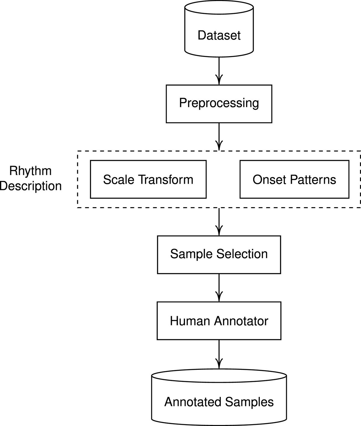
Figure 1
Construction of a set of annotated samples.
We assume that, under annotation budget constraints, if we wish to achieve good beat tracking performance for a given dataset represented by a set of points in the rhythmic feature space, the most informative training samples can be retrieved by an appropriate model of the input distribution. Therefore, our objective is to select samples to be annotated and serve as training data for a state-of-the-art beat tracking model. The cardinality of the resulting labeled set is the labeling budget M, and all remaining samples in the unlabeled set serve as test set for the model. The selected data have to be informative in the sense that, by training the tracking model on the examples in , we should achieve good evaluation results over tracks in . We will abuse our notation and refer to points in , , and as both the tracks and their corresponding features.
Our experiments investigate the importance of selection in low-data scenarios; explore the suitability of two rhythmic descriptors; and evaluate the performance of a TCN-based state-of-the-art beat tracking model trained with data selected according to four different sampling schemes as well as a random selection baseline, on the chosen datasets.
4.1 Features
At the input of our system, we resample the audio tracks to 8000 Hz. A short-time Fourier transform (STFT) of the signal segmented by overlapping sequential 32-ms Hann windows is calculated to produce a 50-Hz frame rate spectrogram. Then, we map the frequency bins to a 40-band mel scale and take the logarithm to represent amplitudes in the dB scale. This mel spectrogram is the base representation from which all rhythm descriptors will be computed.
Scale transform magnitude (STM). To extract this tempo-robust descriptor we follow the original proposal by Holzapfel and Stylianou (2011). First, we compute a spectral flux from the mel-scaled spectrogram. This is possible via first-order differentiation and half-wave rectification of each mel band, followed by the aggregation of all bands. We detrend the resulting onset strength signal (OSS) by removing the local average. Then, we determine the autocorrelation of the OSS with a moving Hamming window of length 8 s and 0.5 s hop. Each frame is transformed into the scale domain by the direct scale transform (Williams and Zalubas, 2000) using an appropriate resolution. Even if preliminary tests with {100, 200, 300, 400} coefficients yielded comparable results on average, we limit our representation to the first 400 scale coefficients (up to scale C = 208) to allow for more complex musical periodicities. At the final step, we average this feature over time, achieving a dimension of 400 for each track.
Onset patterns (OP). The other feature we use to compare audio excerpts is our tempo-sensitive descriptor that draws from the work of Pohle et al. (2009). We will refer to these simply as “onset patterns”, noting that there are a few different implementations of this kind of feature in the literature, as mentioned in Section 3.1. To extract our onset patterns, we first subtract the moving average from each mel channel with a filter length of 0.25 s and half-wave rectify the result. This “unsharp mask” also has an effect of amplitude normalization, since the spectrogram is represented in dB (Seyerlehner et al., 2010). At the second stage, instead of computing modulations with the FFT and mapping the linear scale to log-frequencies (Pohle et al., 2009; Holzapfel et al., 2011), we compute a constant-Q transform (CQT) of the signal in each channel. Like previous work, we define a minimum modulation frequency of 0.5 Hz (30 BPM). Periodicities are described in 25 bins, at five bins per octave, up to 14 Hz. Similarly to Lidy and Rauber (2005); Panteli and Dixon (2016), we average the periodicities over all channels and take the mean feature across all time frames. This results in a descriptor with a dimension of 25.
4.2 Selection schemes
The present study borrows some selective annotation techniques from Su et al. (2023) and Shuyang et al. (2017).
Fast vote-k (VTK). The first selection technique we use is this graph-based selective annotation method, proposed by Su et al. (2023), which determines a set of simultaneously diverse and representative examples given the annotation budget. First, a directed graph G = (V,E) is created where each feature vector in is a vertex in V. Edges E are defined from each vertex to its k nearest neighboring vertices in the embedding space, according to the cosine similarity. We start with and . Then, at every iteration, unlabeled vertices receive a score
where
with r > 1. The score depends on the vertices v from which u can be reached. Each v contributes with its weight, s(v), which is small for v close to vertices already in . These two properties account for representativeness and diversity in the selected set, respectively. At every iteration, a vertex
is moved from to , until . At the first iteration, the algorithm selects the most reachable vertex. We experimented with a few values for k Î {3,5,7,10,15,20,25,30}, but ended up choosing k = 5 as it provided good results across all budgets and datasets.
Diversity (DIV). Another selection technique we use in this work focuses on maximizing the diversity of the labeled set. Following Su et al. (2023), beginning with a random sample, at every iteration i ≤ M the furthest sample from those already in is selected.
Maximum facility location (MFL). We also employ a representativeness selection based on an algorithm by Lin and Bilmes (2009) adapted for the facility location problem (Su et al., 2023). This greedy algorithm optimizes the representativeness of selected samples by measuring the pairwise cosine similarity between embeddings. At every iteration i ≤ M, it selects the most representative example u* as
where cos(∙,∙) is the cosine similarity function and rj is the maximum similarity of xj to the selected samples. At every step, rj, which starts as –1∀j, is updated to .
k-medoids (MED). We include a data selection scheme inspired by the work of Shuyang et al. (2017). We first cluster data with a k-medoids algorithm. Since the medoids returned by this clustering algorithm are the center points that represent local distributions and, at the same time, reside in distinct places of the feature space, we set k = M and directly use the medoids as the set of selected samples . As in the case of vote-k, this selection scheme aims to provide simultaneously diverse and representative examples for training.
Random (RND). All selection schemes are compared to a random baseline: a subset of size M is randomly selected from the dataset to make up .
By leveraging representativeness and diversity, all of the presented selection schemes (except random sampling) are indirectly conditioned by the input data distribution. Since the musical properties (e.g., global tempo, rhythmic patterns, complexity, density) pertinent to our task and features vary differently according to genre and performer, we expect that each distinct dataset might benefit from a different sampling method. In the case of a highly homogeneous dataset, it is perhaps better to annotate a set of more diverse examples. As the data distribution gets increasingly more heterogeneous, representativeness may be weighted more. Moreover, if the dataset is unimodal and highly homogeneous — e.g., composed of a single music genre and displaying little variance in its rhythmic properties —, we would expect to observe little improvement in using smart selection schemes over training on randomly selected data. For less homogeneous (still unimodal) datasets, a proper smart selection should be able to systematically provide better training examples for beat tracking. Finally, in a dataset containing different genres with particular characteristics: (1) A single selection scheme might not be effective for all genres; (2) On average, random sampling will select more examples from the most populated genres, possibly overlooking the less populated ones. In contrast, when genres have the same number of tracks, due to (1) we should not expect large improvements in employing data selection methods.
4.3 Beat tracking model
The main model used throughout our experiments is the TCN-based multi-task model of Böck and Davies (2020), provided in an open-source implementation (Davies et al., 2021). As per the multi-task formulation, it has been shown by Böck and Davies (2020) that it improves the individual estimation of beats, downbeats, and tempo. Since our target is to select good training samples for beat tracking, we ignore both downbeat and tempo estimation heads and consider only beat likelihoods produced by the network. We infer final beat positions with a dynamic Bayesian network (DBN): DBNBeatTracker, from the madmom (v0.17.dev0) package (Böck et al., 2016).
4.3.1 Training
In all experiments, we train the TCN model from scratch with the labeled set output by the data selection stage. We stand on the assumption (Maia et al., 2022) that one can overfit a neural network model for a specific musical genre by training it with few samples, provided the dataset is sufficiently homogeneous in terms of instrumentation, rhythmic patterns, and tempo. Unless otherwise specified, we evaluate the results over the remaining data (). This matches our real-world application, where an end user would employ a small annotation effort (with a budget of M tracks) and train a model on the labeled data hoping to obtain good estimates for the remaining unlabeled tracks. The annotation step is emulated by ground truth annotations.
Both Pinto et al. (2021) and Maia et al. (2022) extracted a single 10-second segment from each musical sample and split it into two disjoint 5-second regions, the first reserved for training and the second for validation. This allowed for more control when tuning the model’s hyperparameters, despite sacrificing half the available information. A similar procedure is followed here: we split each audio track from in half and use the first and second halves as training and validation, respectively; test data are not cut. In all cases, we set the network learning rate to 0.005, with a decay factor of 0.2 if no improvement in the validation loss is observed after 10 epochs. We train for at most 100 epochs, with early stopping enabled when training stalls for 20 epochs.
4.4 Datasets
We use three sets of audio tracks to evaluate our methodology under different conditions. Two of them are associated with distinctively percussive Afro-rooted Latin American music traditions that motivate the main problem of this article. The first one is the Candombe dataset (Nunes et al., 2015; Rocamora et al., 2015), which contains 35 recordings of candombe drumming (2.5 h in duration) featuring three to five drummers performing different configurations of the three candombe drums (piano, chico, and repique). The second dataset comprises the ensemble recordings from the BRID dataset (Maia et al., 2018): 93 tracks of about 30 s each featuring two to four Brazilian percussionists playing characteristic rhythm patterns of mostly samba, partido-alto, and samba de enredo. In total, 10 instrument classes are arranged in typical ensembles of Brazilian music — samba in particular. We note that both datasets were collected with the consent of the musicians. Furthermore, we also explored the Ballroom dataset (Gouyon et al., 2006; Krebs et al., 2013), a standard of the beat tracking literature. Unlike BRID and Candombe, it consists of many distinct genres and was selected to serve as a counterpoint in our investigation. It includes 698 tracks of eight ballroom dance genres (cha-cha-cha, jive, quickstep, rumba, samba, tango, Viennese waltz, waltz) of 31 s on average. To allow a direct comparison of results across all datasets, candombe tracks were segmented into 276 non-overlapping 30-second excerpts. All genre labels were ignored in our experiments.
A deeper analysis of the characteristics of each dataset is presented in Section 5.1.
4.5 Evaluation
Using the implementation provided in the madmom package, we evaluate the beat prediction results through the F-measure (Dixon, 2007), which is the harmonic mean between the proportion of correct estimates (precision) and the proportion of correctly estimated beats (recall), with the usual tolerance of ±70 ms around annotations.
5 Experiments and Results
5.1 Dataset homogeneity
Preceding our experiments, we investigate tempo and rhythmic variability of tracks from each dataset.
Figure 2 presents the datasets’ global tempo distributions smoothed by a Gaussian kernel density estimation technique. Candombe exhibits a slim distribution, averaging 132 BPM (8 BPM standard deviation), while BRID is approximately bimodal, whose peaks at 95 and 130 BPM can be respectively associated with samba/partido-alto and samba de enredo subgenres. Unsurprisingly, Ballroom’s multi-genre characteristic is disclosed by multiple modes; individual distributions are described by Krebs et al. (2013).

Figure 2
Global tempo distributions.
A representation of the rhythmic patterns across all datasets is displayed in Figure 3. The scale transform magnitudes (STM) were obtained from each track following the procedure described in Section 4.1. Then, manifold learning with UMAP (McInnes et al., 2018) was used to reduce the feature space dimension from 400 to 2 using the cosine distance as a metric. A major advantage of UMAP over other commonly used dimensionality reduction approaches like t-SNE is that it can better represent global data structure while preserving local neighborhoods (McInnes et al., 2020). UMAP diagnoses that Ballroom patterns mostly lie in regions whose local dimension is estimated as high. That means they are less accurately represented in this embedding, and thus display greater rhythmic variation than can be represented in two dimensions. Candombe has a small set of outliers but is mostly represented in a compact structure, whereas BRID, despite having fewer examples, is more spread out in the embedding space. Interestingly, the subset of Ballroom located near BRID and Candombe is mostly composed of tracks from the “Samba” genre, with few examples of “Jive”.
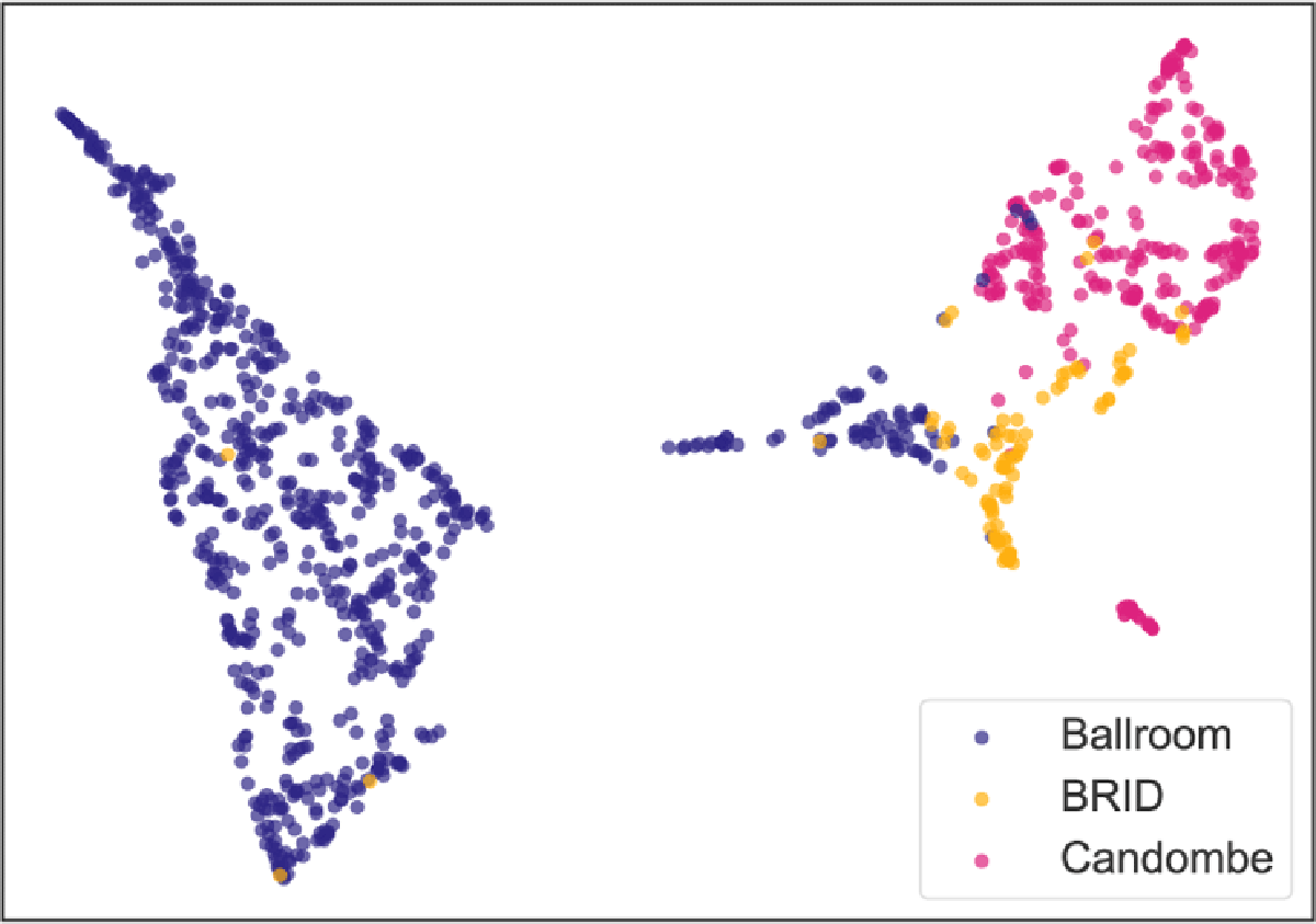
Figure 3
STM features embedded by UMAP (cosine metric, n-neighbors = 15, min-dist = 0.1).
5.2 State-of-the-art results without selection
To contextualize the outcomes of our experiments, we present in Table 1 the beat tracking performances on BRID and Candombe of models using the architecture of Böck and Davies (2020) under three different training schemes:
Table 1
Performances of the state of the art (without data selection): mean (standard deviation) in %.
| BEAT F-MEASURE (%) | ||
|---|---|---|
| MODEL | BRID | CANDOMBE |
| Pre-trained (Maia et al., 2022) | 60.0 | 15.9 |
| Fine-tuned (3 min) | 93.4 (3.4) | 98.2 (1.1) |
| Trained from scratch (all) | 98.9 (1.2) | 99.8 (0.3) |
“Pre-trained”: results of the TCN model from our former work (Maia et al., 2022) — network trained on 38 h of Western music material from six datasets (including Ballroom), and tested on the entire BRID and Candombe datasets;
“Fine-tuned”: the “pre-trained” model that we fine-tuned for each dataset with 3 min of randomly selected data (tracks were split in half for training and validation), tested on the remaining data. We used 10 random selections, 30 training seeds, and the fine-tuning parameters of Maia et al. (2022);
“Trained from scratch”: the TCN model initialized randomly and trained for each dataset on full 30-second tracks, using an eight-fold cross-validation scheme. One fold was used for testing, one for validation, and six for training. The training was repeated until all folds had been used for testing. For training parameters see Section 4.3.
5.3 Experiment 1: Does sampling matter?
In this first experiment, we assess the dependence of beat tracking performance on random training sets in low-data scenarios. Depending on the annotation budget, it is often not feasible to explore all possible training sets. By choosing to focus on the BRID dataset, which has the smallest number of tracks of all datasets, we are able to survey a larger proportion of all random combinations. In this sense, we set the annotation budget to M = 4 tracks, which yields around 3 million possible combinations of four distinct elements out of 93 total tracks. Then, we select 1000 of these combinations, ensuring that all tracks in the dataset are about equally represented overall. We use each unique combination to train/validate the TCN model, which we evaluate over the complementary test set of 89 files. We repeat each training 30 times with different randomly initialized weights and seeds.
Figure 4 shows the averages and standard deviations for the performances of all trained models in ascending order of mean beat F-measure. We note that mean beat F-measures range from 46.5% to 90.1% depending on the training set, with the 5th and 95th percentiles corresponding to 61.0% and 85.4%. A mean F-measure of 74.4% is achieved on average.
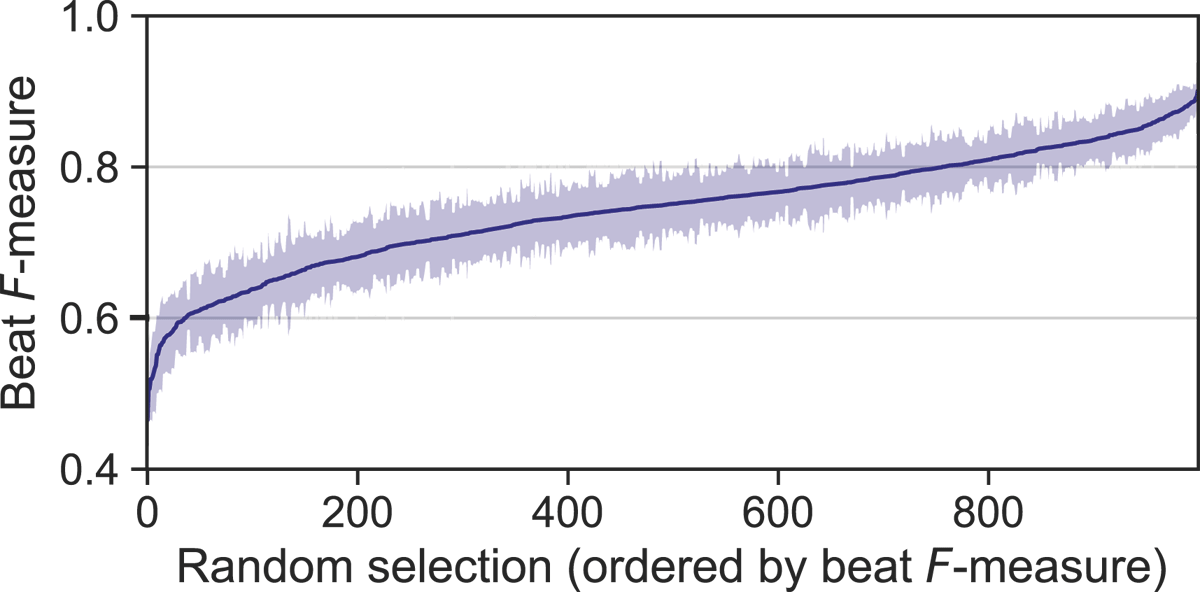
Figure 4
Results for Experiment 1. Random data selections on the BRID dataset ordered by mean F-measure, showing standard deviations (shaded area).
This experiment shows the importance of adequate data selection for the TCN model when dealing with low-data training scenarios. With an annotation budget of M = 4 tracks, we observe a considerable improvement of about 16 percent points over the average case and 44 percent points over the worst case when estimating beats on the BRID dataset.
5.4 Experiment 2: Feature structure
In this second experiment, we investigate the local structure of the feature space generated by each rhythm description feature (STM and OP) and its capability of conveying meaning for the data selection scheme. For this purpose, considering the distribution of a dataset in the feature space, we analyze the performance of the TCN model when trained with points sampled from different regions around single test tracks. We hypothesize that regions closer to the test sample provide better training examples, thus yielding better beat tracking results. Again we set the annotation budget to M = 4, but this time we observe all datasets separately.
The regions are limited by concentric hyperspheres centered at each test sample, whose radii depend on the distribution of the dataset in the feature space. If Q1, Q2, and Q3 are the first, second, and third quartiles of the pairwise feature distances of points in the dataset, respectively, we define , , and , the regions in increasing distance from a given test file, xj, as
where i ≠ j. We also define the set of remaining points, which lie outside the largest hypersphere, as
Figure 5 exemplifies the computation of these regions from a normal data distribution in a two-dimensional space using the Euclidean distance. In practice, we use the cosine distance, i.e.,
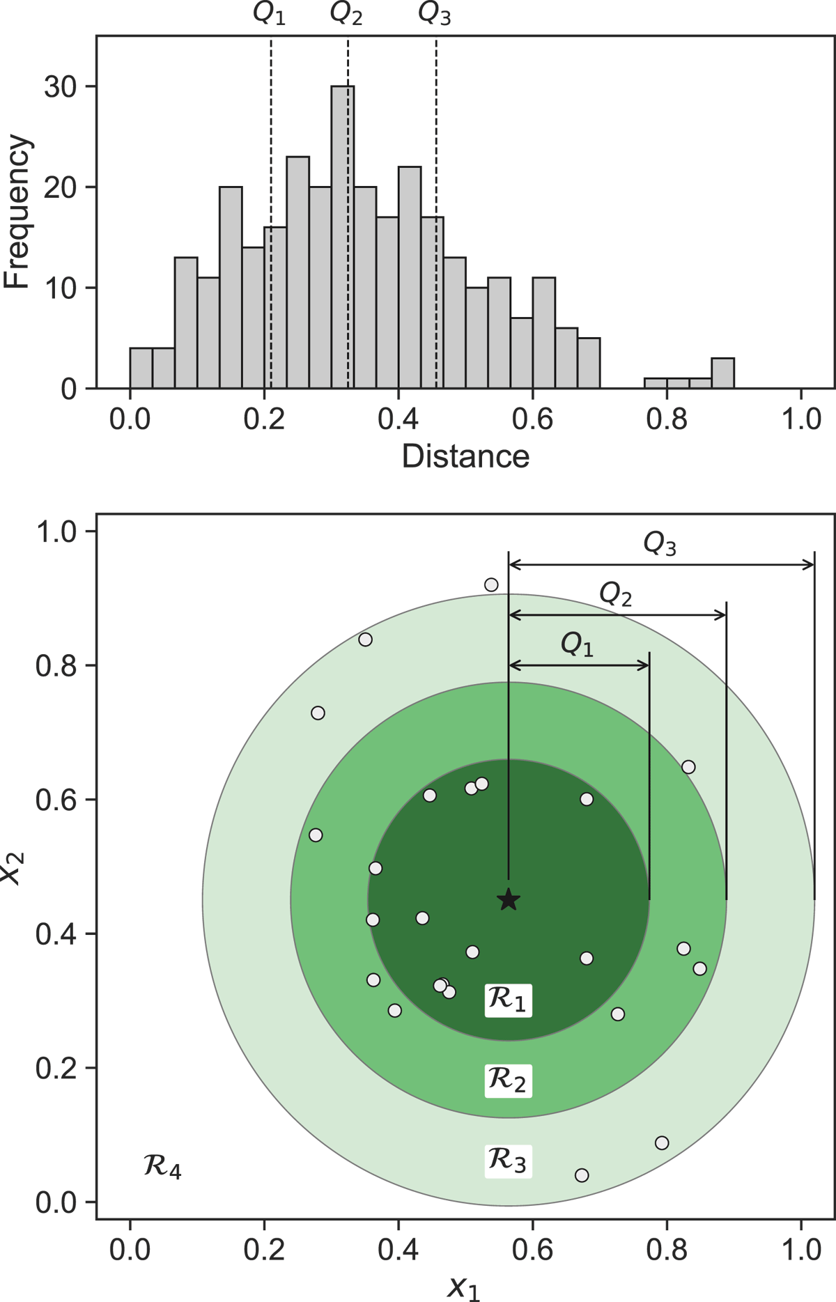
Figure 5
Example of pairwise feature distance frequencies and regions surrounding a single test sample (star) from a normal data distribution. The distance distribution (top) defines quartile regions in the feature domain (bottom).
Once all regions are determined for a reference track, xj, we can compare how well models trained and validated on sets of randomly selected points from each region perform on the test set . We repeat this process for all points in the dataset that contain at least M = 4 examples in each of its regions. This way, we end up training four different models per reference sample. Once again, we repeat the training process 30 times, with different seeds, keeping the same training sets.
The results of this experiment are presented in Figure 6. We show the average F-measure gain across all models when using points from each region over using points from the farthest region . Mathematically, if is the F-measure of a model trained on points from the region around sample , then
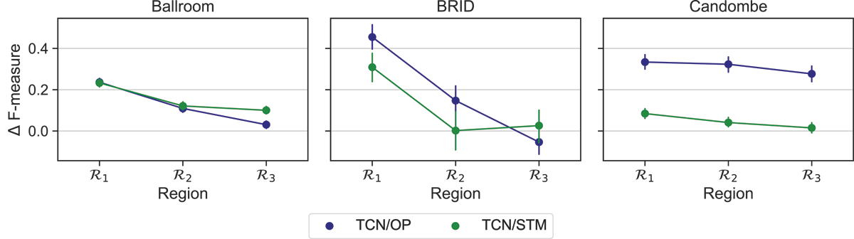
Figure 6
Results for Experiment 2. Average beat F-measure gains (95% confidence interval) w.r.t. sampling from .
where , for i Î {1,2,3}. For all datasets, we observe that the best models are trained on points from the closest regions , independently of the feature. We may also compare the gain from using over , for example. Using a set of immediate neighbors leads to significant gains in BRID, as shown by the substantial difference between results in the two regions. In Ballroom this gain is much smaller, and in Candombe it is almost negligible. It is worth noting that for Candombe, the absolute beat F-measure values are 91.7% and 96.4% for STM and OP, respectively, in . These compare to 62.6% and 65.3%, respectively, for the same region in BRID. This means that there is more room for improvement in BRID than in Candombe. Without forgetting that the definition of these regions depends on the data distribution of each dataset, we can say that data selection must be more important in the former than in the latter.
We have shown with this experiment that one can train beat tracking models that are better able to generalize to recordings in local neighborhoods defined in the space of the rhythmic features. This is a promising result that suggests that these features can be employed to retrieve informative samples.
5.5 Experiment 3: Sampling strategies
In this experiment, we examine all combinations of rhythm description and sample selection techniques across different annotation budgets; and evaluate the beat tracking performance of a TCN model trained on the selected data and tested on the remainder of each dataset. This experiment represents the use case of our proposal. As we mentioned before, the main difference to the real-world scenario is that we use ground-truth annotations instead of asking for a human to provide labels for . We wish to investigate how much a sampling strategy can improve tracking performance against random sampling. Naturally, this depends on the properties (e.g., tempo and rhythm pattern distributions) of each dataset as well as on the specified annotation budget.
For BRID and Candombe, we vary the annotation budget from 4 to 14 samples (in steps of 2), i.e., about 2–7 min of annotations. Since Ballroom has many more tracks (about 7.5 and 2.5 times more than BRID and Candombe, respectively) and genres, we use larger budgets for this dataset, M = {10,16,22,28,34,40} (~5–20 min), i.e., around 2.5 times more data. As in all experiments, training files are split in half for training and validation purposes. Regarding the selective sampling techniques, we observe that MFL and VTK are deterministic and as such always provide the same labeling sets. DIV and MED depend on a random initialization. However, we noticed that a considerable number of files (usually M–2 or M–1) were repeatedly selected over multiple executions of the DIV sampling process, which means that, especially for larger budgets, it is nearly deterministic. In the case of MED, smart initialization and multiple runs were used to obtain a more robust clustering. Once these sampling techniques have provided consistent results, we use them to select one set of training examples for each combination of dataset, labeling budget, and feature representation. Finally, for the random baselines (RND), 10 random selections of M files were carried through for each dataset–budget pair; these are used to indicate the expected performance of the TCN model. For each data selection, we repeat the training process 30 times with different seeds.
Beat tracking performance (means and standard deviations) is summarized in Table 2. Looking at these results, we notice that, in most cases, selective sampling techniques are consistently better than random sampling across all budgets, although the best feature–selection pair greatly depends on the dataset and training size. In particular, STM+MFL stands out as the best setup for Ballroom, closely followed by STM+MED and OP+MED, showing gains of up to 5.2 percentage points (M = 16) over the random baseline. In extremely low-data scenarios, OP+MED produces the best results for BRID, with an 18.3 point increase over random at the smallest budget, although STM+MED and OP+MFL provide good results as well. In both Ballroom and BRID, diversity sampling gives worse results than random for STM (–4 percentage points on average). DIV is also worse than RND with OP in Ballroom (almost –5 points on average), and inconsistent in BRID when paired with the same feature representation. Finally, the RND baseline performance in Candombe is already very high (94.0–96.8%), which leaves little room for improvement in this case. However, except for the two smallest budgets, OP+DIV provides moderate gains for this dataset (2.3 points on average).
Table 2
Results for Experiment 3: mean value (standard deviation) in %. In boldface, the best-performing selective sampling technique given M (budget) and feature, for each dataset; in gray, the best-performing setup in each dataset–budget pair. Sampling techniques: diversity (DIV), k-medoids (MED), maximum facility location (MFL), vote-k (VTK), random (RND).
| BEAT F-MEASURE (%) | |||||||||||
|---|---|---|---|---|---|---|---|---|---|---|---|
| ONSET PATTERNS (OP) | SCALE TRANSFORM MAGNITUDES (STM) | RND | |||||||||
| DATASET | M | DIV | MED | MFL | VTK | DIV | MED | MFL | VTK | ||
| Ballroom | 10 | 69.5 (2.3) | 77.2 (2.0) | 76.7 (2.5) | 74.8 (3.0) | 66.0 (2.9) | 77.4 (2.0) | 75.5 (1.9) | 75.2 (1.8) | 72.5 (4.5) | |
| 16 | 72.3 (2.7) | 81.1 (1.1) | 78.4 (2.3) | 77.9 (3.6) | 76.7 (1.9) | 80.4 (1.1) | 82.1 (1.1) | 78.8 (0.9) | 76.9 (3.2) | ||
| 22 | 74.1 (1.5) | 82.2 (1.1) | 82.0 (1.2) | 79.7 (1.0) | 79.8 (2.3) | 84.1 (0.7) | 85.4 (0.6) | 81.3 (1.4) | 81.1 (2.8) | ||
| 28 | 79.0 (1.5) | 83.8 (0.7) | 83.0 (1.2) | 81.0 (0.9) | 77.8 (2.4) | 84.7 (0.8) | 85.9 (0.5) | 83.2 (0.8) | 83.5 (1.5) | ||
| 34 | 79.8 (1.0) | 85.6 (0.8) | 84.3 (0.9) | 83.0 (1.2) | 78.1 (2.0) | 85.7 (0.8) | 85.8 (0.6) | 85.3 (0.8) | 84.6 (1.4) | ||
| 40 | 81.1 (1.4) | 85.2 (0.9) | 84.9 (1.0) | 83.5 (0.9) | 79.3 (1.8) | 84.8 (1.0) | 85.2 (1.3) | 85.2 (0.5) | 85.2 (1.4) | ||
| BRID | 4 | 83.9 (4.4) | 91.0 (2.2) | 88.7 (3.8) | 81.8 (3.3) | 66.7 (8.2) | 86.0 (2.7) | 76.3 (9.5) | 75.0 (4.1) | 72.7 (8.4) | |
| 6 | 75.9 (5.3) | 90.9 (2.8) | 89.2 (4.2) | 86.7 (1.7) | 72.5 (4.9) | 88.2 (5.7) | 82.9 (3.4) | 84.2 (4.6) | 76.3 (8.3) | ||
| 8 | 81.4 (5.0) | 89.9 (3.8) | 89.6 (3.0) | 90.6 (2.1) | 87.4 (3.1) | 82.8 (4.3) | 89.4 (2.4) | 91.2 (1.9) | 78.2 (8.4) | ||
| 10 | 84.3 (4.6) | 93.7 (1.9) | 94.9 (1.4) | 89.1 (1.2) | 79.6 (3.7) | 91.3 (2.5) | 89.2 (2.6) | 94.3 (1.7) | 82.7 (8.7) | ||
| 12 | 90.5 (1.7) | 93.3 (1.7) | 94.0 (6.0) | 91.0 (1.7) | 80.7 (4.7) | 89.6 (4.8) | 90.7 (2.6) | 94.1 (1.5) | 85.5 (6.9) | ||
| 14 | 87.9 (2.3) | 92.7 (2.0) | 94.1 (1.9) | 91.2 (1.4) | 80.7 (3.3) | 91.4 (3.2) | 91.5 (2.2) | 95.8 (1.1) | 89.3 (4.7) | ||
| Candombe | 4 | 81.2 (7.4) | 91.6 (2.5) | 82.8 (3.7) | 90.3 (2.5) | 89.5 (2.8) | 90.5 (4.5) | 94.9 (0.8) | 93.7 (1.1) | 94.0 (3.7) | |
| 6 | 83.7 (13.7) | 95.2 (2.6) | 91.7 (1.7) | 93.2 (1.8) | 90.3 (2.4) | 96.4 (0.6) | 95.1 (0.7) | 95.7 (1.0) | 95.0 (1.8) | ||
| 8 | 97.0 (1.3) | 96.1 (1.7) | 92.5 (1.9) | 92.5 (1.0) | 94.6 (2.6) | 96.0 (0.7) | 95.2 (0.8) | 96.0 (0.7) | 95.2 (1.5) | ||
| 10 | 98.2 (1.2) | 96.5 (1.2) | 94.4 (1.5) | 93.0 (0.7) | 96.8 (0.7) | 96.2 (0.6) | 96.3 (0.5) | 96.0 (0.8) | 95.9 (1.7) | ||
| 12 | 99.0 (0.3) | 95.4 (2.6) | 96.8 (1.0) | 93.8 (0.9) | 98.2 (0.7) | 96.1 (0.6) | 96.3 (0.6) | 96.1 (0.6) | 96.5 (1.5) | ||
| 14 | 99.2 (0.2) | 98.8 (0.1) | 97.1 (1.0) | 93.8 (0.5) | 98.4 (0.4) | 96.1 (0.6) | 96.2 (0.5) | 96.1 (0.5) | 96.8 (1.5) | ||
The general conclusion is that using sampling techniques can provide better training examples for the TCN model, since most feature–selection setups are shown to outperform the random baseline. This performance gain is typically larger the smaller the annotation budget. We also note that a smart data selection can reduce the standard deviation of the results, leading to more stable solutions than those obtained through random selection. Unsurprisingly, since there are many possible dataset configurations (e.g., highly homogeneous, highly heterogeneous), there is no optimal setup. We discuss a set of recommendations based on our results in the following.
6 Discussion
In this research, we have studied the influence of data selection on the effectiveness of beat tracking systems that are trained using a limited amount of data. We found out that selective sampling techniques, which take into account the data distribution, can significantly improve beat tracking performance compared to a random selection baseline, while also reducing its variance. This improvement was observed even when working with small training sets. The baseline results are consistent with those of our previous research (Maia et al., 2022), which used the same datasets but did not employ any specific selection scheme.
We noticed that, in general, when the size of the training set is smaller, performance improvements tend to be more significant. This is mainly due to two reasons. Firstly, it becomes more challenging to improve performance when the results are already very good, which is usually the case with larger annotation budgets. Secondly, with less data, each selected sample contributes proportionally more to what the model sees during training, thus having a greater impact on beat estimates, e.g., changing a single sample in a set of four is more critical than changing it in a set of 20 samples.
Regarding feature representations, it is currently unclear which is preferable, as both OP and STM allowed for good training samples to be selected. Initially, we had a suspicion that OPs, which encode tempo information, would produce better results than STM in general, given that the TCN model is sensitive to the tempo distribution of the dataset (Böck and Davies, 2020). However, it should be noted that, at the post-processing DBN stage, the tempo is dissociated from the rhythmic pattern and separately encoded in the state variable. Additionally, the difference in dimensionality between the two features cannot be ignored. Further investigation is needed to determine which representation is more effective.
This study has also examined the results of sample selection on different datasets. Although our work primarily focuses on single-genre datasets from Afro-rooted traditions, we highlight the moderate performance gains observed in Ballroom, which is highly diverse with various genres, meters, and patterns (see Section 5.1). We then turn our attention to the two main datasets, Candombe and BRID. Candombe, which displays the smallest tempo range and little pattern variability, benefited less from tailored sets of training examples. However, we note that models trained on random selections already accurately track Candombe excerpts, which means there is less room for improvement. On the other hand, BRID, which is less homogeneous, seemed to profit the most from sample selection. It is yet to be determined how exactly these two characteristics — tempo and rhythm — affect the impact of selection in each dataset, and whether general rules could be established to inform when selective sampling is most beneficial. We underscore that OP+DIV (which maximizes diversity) and STM+MFL (which maximizes representativeness) were the best-performing setups for Candombe (most homogeneous) and Ballroom (most heterogeneous), respectively. For BRID, on the other hand, MED and VTK — both making a compromise between diversity and representativeness — were the better sampling schemes.
Finally, it is worth comparing our results with the state-of-the-art procedures discussed in Section 5.2. First, we observe that our results consolidate the idea of adapting to challenging music already expressed by Pinto et al. (2021); Yamamoto (2021); Maia et al. (2022). We saw in Experiment 1, under a restrictive scenario (2 min of training data), that a large majority of the adapted models greatly surpassed the “pre-trained” model (Table 1), which was trained on hours of data from standard datasets. This improvement was more evident when data selection was carefully planned (Table 2). Our selective sampling strategy proved to be much more effective than the random baseline, as we achieved results that are very close to the “trained from scratch” model (which we consider a “full-dataset” performance). For example, in BRID, with the same 2 min of data, there is only a 7.9 percent difference, while RND is behind by 26.2 points. It is also worth mentioning that our selective sampling approach is comparable to transfer-learning-based procedures. With a budget of M = 6 samples (3 min of annotations), we have obtained results that are on par with the “fine-tuned” models for Candombe and BRID, with only slight differences of –1.8 and –2.5 percent points, respectively, considering the best feature–selection pairs, but with lower variability. We must note that our approach is not only affordable but should be considered more general, as pre-trained networks may have been trained on data that is not relevant to the object of study, which could compromise the stability of the results.
7 Conclusion
The objective of this study was to propose an effective methodology for selecting training samples in small data scenarios for a beat tracking model, considering the user’s perspective. In this regard, we have presented a framework that combines tempo-sensitive and tempo-robust rhythmic features with selective sampling techniques that exploit the internal distribution of the data. Our system projects the dataset into the feature space and outputs a selection of meaningful examples, which are subject to a user-informed annotation budget. In real-world applications, the user is then given this labeled set and produces the corresponding annotations. Finally, a TCN-based state-of-the-art tracking model is used to estimate beat positions for the remaining tracks in the dataset.
The experiments conducted have highlighted the importance of carefully selecting the training data for the TCN model. Our suggested framework has shown better results as compared to random data selection, as evidenced in our main experiment (Section 5.5). The experiments also revealed that there are complex non-linear interactions between the training set and test set sizes, rhythm properties, features, and sampling techniques. Nonetheless, we can confirm that the results align with our intuition on utilizing diversity and representativeness in the selection (Section 4.2).
We would like to mention that our analysis of each dataset has been limited to two musical parameters: global tempo and rhythmic patterns. Going forward, we could synthetically generate data and create a diverse collection of datasets that vary not only in those but also in other musical aspects (e.g., tempo and pattern changes within each track, pattern complexity/density), and follow a similar training procedure. This would allow a more in-depth analysis of those complex interactions. It would also be interesting to investigate the results on other challenging music datasets, e.g., SMC (Holzapfel et al., 2012) and Hainsworth (Hainsworth and Macleod, 2004).
We hope our proposed methodology can help alleviate data annotation bottlenecks, especially when it comes to culturally diverse music datasets. Even though the datasets used in this study are very percussive, the same framework should also work for music with little to no percussive content (Holzapfel and Stylianou, 2011). Furthermore, we believe that a similar pipeline could be utilized for efficient data selection in other supervised learning problems in MIR. This includes mood and genre classification as well as other retrieval tasks.
Data Accessibility Statement
Our code is available at https://github.com/maia-ls/tismir-beat-2024.
Funding Information
This work was partially supported by the Coordenação de Aperfeiçoamento de Pessoal de Nível Superior – Brasil (CAPES) – Finance Code 001; the Conselho Nacional de Desenvolvimento Científico e Tecnológico (CNPq) – grant nos. 141356/2018-9 and 311146/2021-0; and by the Sistema Nacional de Investigadores – Agencia Nacional de Investigación e Innovación (SNI-ANII).
Competing Interests
The authors have no competing interests to declare.
Author Contributions
Lucas S. Maia was the main contributor to writing the article, running experiments, and analyzing results. Magdalena Fuentes and Martín Rocamora helped with the experimental setup by preparing the necessary code. Magdalena Fuentes and Luiz W. P. Biscainho co-supervised the work. All authors actively participated in the study design, contributed to writing the article, and approved the final version of the manuscript.