
1. Introduction
An increasing proportion of people rely upon streaming services to listen to music, and large amounts of detailed, individual data collected by these services are becoming available to scientists. These data open the door to an improved understanding of spatial and temporal dynamics related to music consumption, such as the long-term evolution of people’s listening behavior through the course of their life, or the geographical spread of different songs, artists and music genres at different periods of time. However, in order to study such high-level dynamics, it is necessary to have quantitative tools that are able to capture and expressively summarize these enormous amounts of listening data and musical preferences produced by millions of users.
Quantitative research on people’s musical taste spans over many scientific disciplines. From a sociological standpoint, musical taste has been long studied as a self-declared, differentiating feature among individuals and social groups (Bourdieu, 1984; Peterson, 1992; Bryson, 1996). Psychological studies have been investigating correlations between musical preferences and personality traits (George et al., 2007; North, 2010). More recently, the concept has been used in the music recommender systems literature, as the distinctive part of the musical space from which a user is likely to enjoy a recommendation (Laplante, 2014; Ferwerda and Schedl, 2014; Uitdenbogerd and Schyndel, 2002). While in its general understanding, musical taste is an individual’s set of musical preferences, when it comes to the literature we observe conflicting approaches that can be broken down into three dichotomies. The first one lies in the empirical data supporting the research – declarative information collected in questionnaire surveys or interview-based research, versus interaction traces assumed as implicit and explicit preferences that can be retrieved from online activity logs. The second dichotomy is related to the “resolution” of the information at hand: either aggregated (generally at the level of music genres), or directly at the “atomic” level of musical items, namely songs, albums and artists. Finally, the third dichotomy of musical taste is the focus on either its distinctive features – what in their taste makes individuals or groups different from one another? – or the focus onto its essence – what, among an individual’s appreciations, best sums them up?
In recommendation, usage data and explicit preferences collected by platforms are used to derive average “taste profiles” from which new items can be sampled and proposed. There are also examples of recommender algorithms that treat each user as a mixture of profiles (Vargas and Castells, 2013), or which use contextual cues to modulate recommendations (Liang et al., 2018). This is somehow a reductionist vision of what makes personal taste, as it assumes that it can be summarized. It can also be said that it is an operational definition that basically reverts the problem of providing a comprehensive definition: in a recommendation setting, taste is what can be leveraged to make relevant recommendations. It is also interesting to notice that it is not consistent with the relational approach that is used in sociology, where taste and distaste have traditionally been represented as a set of preferences that distinguish one social group from another – social groups being constituted on the basis of the economic, educational and cultural capital of individuals (measured through variables such as their occupation, their parents’ occupations, or the highest degree they obtained). In the end, practitioners of both fields share the common objective to capture what distinguish people when it comes to their musical preferences. People engineering recommender systems are more interested in building systems able to predict items that people will like, while sociologists of taste are interested in finding what are the variables that best explain social differences in taste and distaste. Both are interested in building a system able to summarize and predict an individual’s musical preferences.
Getting back to the tools required to study high-level dynamics of music listening in societies, it would be extremely useful to be able to capture some kind of “fingerprint” of an individual’s musical preferences. From a computational perspective, a good fingerprint should possess different desirable properties. It should be expressive, and provide a good summary of the diversity of the music appreciated by the user. It should also be concise, i.e. be composed of as much information as necessary but not more. Most of all, it should be able to serve as a fingerprint, i.e. a signature able to identify a user among others. These properties may prove to be difficult to achieve simultaneously via a single fingerprinting procedure, and in the remainder of this paper we will investigate this question experimentally.
More precisely, we are interested in formalizing and comparing different views of taste, and in order to do so we will formalize these views in a fingerprinting problem, that is, an information summarization problem that we will study by considering two distinct sets of constraints. The first set is designed to capture a user’s identity, in the sense of its identifiability among others. Identifiability through music is also a topic of interest for privacy purposes: with explicit preference data being ubiquitous on the open internet, measuring to what extent individuals can be uniquely identified through their portfolio of content preferences is important. We will try to answer the following questions:
RQ1: To what extent are users identifiable through their online activity data (favorite items and streaming history)?
RQ2: What information (content and size) is needed to identify people?
We wish to answer these questions by assigning users a so-called fingerprint – a small set of items that allows us to identify users in a unique way.
The second set of constraints is expressed as a representativeness problem, i.e. finding the essence of one’s preferences. We will adopt a data-driven approach, and propose one formalization of what a taste fingerprinting procedure could be, similar to a classic recommendation setup, and evaluated through a prediction task. We will then confront the two sets of constraints, in order to answer the following question:
RQ3: Are the items that make one’s preferences unique representative of these preferences?
In our experimental setup, we will use a dataset containing the explicit preferences (e.g. artists and songs that have been deliberately liked by users, by clicking on a heart-shaped icon) of about 1M users of a music streaming platform, as well as liked and streamed artists for another 50K users.
The remainder of the paper is organized as follows: in the next section we provide an overview of the previous work in social science and recommender systems related to the measure of the notion of “musical taste”. Section 3 presents the data, while sections 4 and 5 present the experiments we conducted and the results we obtained for the fingerprinting problem with the two different sets of constraints. Section 6 concludes the paper.
2. Related Work
In order to measure and quantify musical taste, we need to understand all the aspects that this term can describe. In this section, we make an overview of characteristics necessary to study musical taste through three axes. First, we dive through existing ways of collecting data. Then, we discuss different representations of music. Finally, we overview two diverging views of musical taste found in the literature – as an attribute of distinction among others, or as a set of characteristics of our preferences.
2.1 Music preference data collection
In sociology and psychology, collecting declarative data about musical preferences and consumption habits through surveys and interviews is common. Interacting directly with the respondents is advantageous for several reasons. The use of a Likert scale for instance allows to have a deeper understanding of how much respondents do or do not like certain music (Peterson, 1992; Bryson, 1996). Information about context of music consumption can be collected (DeNora, 2000), as well as sociodemographics, that can then be crossed with declared music preferences (Bourdieu, 1984; Peterson, 1992; Bryson, 1996; Coulangeon, 2017; Lahire, 2008). However, the sample of surveyed individuals is usually limited, and the results can be biased as such surveys are often run either in a specific country, or on a specific social group, like students for example (Delsing et al., 2008; Brown, 2012; Langmeyer et al., 2012). Additionally, the respondents may find it difficult to realistically assess what music they like to listen to and in what proportion. Flegal et al. (2019) show that some people struggle to estimate their own weight, and we can imagine that there might be a gap between declared preferences and the music that respondents actually listen to. For instance, it is possible that people tend to overstate listening to some more socially appealing music genres, and neglect to mention the less socially accepted music they like.
On the other hand, recommender systems mostly rely on observable data, often collected as traces of activity in online platforms. The huge amount of collected data should allow a good understanding of the users’ listening practices, and even though the context or sociodemographics are not explicitly collected, the data could be used to deduce some implicit information. For example, Way et al. (2019) estimate the relocation of certain users by analysing the changes in their IP address. However, the collected traces are often ambiguous and considered as implicit markers of preference (or negative markers, in the case of skipped songs for example) (Oard and Kim, 1998; Majumdar et al., 2009).
A way to have a complete understanding of people’s preferences would be to cross observable and declared data. This idea has been recently proposed (Cura et al., 2022) in the form of “augmented interviews” leveraging digital traces to inform and assist social science researchers conducting interviews.
2.2 Music representation
In order to quantify musical taste, one must first be able to segment the musical space itself. For this, music preferences can be assessed either directly using music items, like artists or songs (Bourdieu, 1984), or through the mediation of aggregated categories. In surveys, for the sake of brevity, preferences are often collected via set of music genres (Peterson, 1992; Bryson, 1996; Coulangeon, 2017). Even though representing music through genres may seem obvious, it is important to keep in mind that no universal genre taxonomy exists, thus using genres to depict people’s musical taste can create bias (Sordo et al., 2008). Music can also be classified by so called “mood”, that can be identified either through audio features (Soleymani et al., 2015; Delbouys et al., 2018) or through declared data (Rentfrow and Gosling, 2003). Bogdanov et al. (2013) used audio features in order to depict people’s musical taste.
2.3 Distinction and essence
In the literature, taste is often defined as a set of traits that distinguishes us from others and marks our individuality. In sociology, musical taste has long been studied in association with social class belonging. Bourdieu (1984), Peterson (1992), Bryson (1996) and Coulangeon (2017) show the connection between musical preferences and social class – people present their taste as a mark of belonging to their “in-group” while differentiating themselves from an “out-group”. Similar conclusions have been found in psychological studies, like Hargreaves et al. (2006), who studied adolescents and how they use music to build their social identity. Later, Lahire (2008) studies intra-individual behavioral variations and emphasizes that most people have preferences that are not typical for their social group, and thus taste is an individual characteristic. The need people have for distinctiveness or “uniqueness” in order to self-identify has been studied in psychology as well (Fromkin and Snyder, 1980).
The notion of distinctive identity is also reminiscent of that of digital identifiability, that is, to what extent people’s behavior (and digital traces of it) can be used to uniquely identify individuals. For example, De Montjoye et al. (2013) use mobility data and show that four spatio-temporal points are enough to uniquely identify 95% of individuals. Narayanan and Shmatikov (2008) use the Netflix Prize dataset to de-anonimize users through the movies they have watched on the platform. They show that 5–10 movie ratings are enough to identify most users. These studies present an extreme form of distinction, where each individual is literally identified in a unique way among all others. However, no such experiment has been run on music streaming data.
An alternate definition of musical taste would be a set of factors that characterize listening behavior of an individual. This is typically the definition implicitly adopted as the core principle for designing recommender systems, where the goal is to understand the essence of the user’s preferences in order to suggest them similar music. Two main approaches exist in recommender systems. In collaborative filtering, the idea is to assign users a descriptive vector, or embedding, based on similarities between other users. The same process is applied to determine the similarity between items. This can be done through matrix factorization (Koren et al., 2009) based on either implicit feedback, like streaming activity logs, or explicit feedback such as users’ collections of favorite items and playlisting of songs. Content-based recommendation, on the other hand, tries to define the items’ features that a user will respond positively to. These features can be represented by various tags (Pazzani and Billsus, 2007) that can be automatically computed based on audio features in the case of music (Cano et al., 2005; Van den Oord et al., 2013; Schedl et al., 2015) or social tags that can furnished by music providers or collected from the Web (Eck et al., 2007).
As concluding remarks, one may point out that the literature is rich with attempts to characterize musical taste, but they seem to be hard to reconcile, as they diverge on several key aspects. The first one is quantization of the musical space, the second being the data collected and the analysis methods. But most importantly there are conflicting hypothesis on the very nature of an individual’s musical taste. While social sciences emphasize the importance it bears in the construct of one’s self-identity, the emerging field of recommender systems assumes a form of homogeneity, even predictability of one’s taste.
This raises a series of open questions: to what extent is it possible to identify people based on their musical preferences? Assuming there are distinctive traits in one’s musical consumption, are these truly reflective of their global behavior?
3. Dataset
3.1 Overview
For this study, we work with data obtained from the music streaming service Deezer,1 that currently counts about 16M active subscribing users worldwide and has a catalog of 90M tracks. First, we collected explicit feedback data (i.e. “likes”) from 1M randomly selected users, who have been active during October 2022. Let us call this data sample DL. Users can explicitly “like” songs, albums, and artists which then appear in their “favorites” collection. As of the date of the data collection, among these 1M users 87.1% of them had explicitly liked at least one artist, and 88.9% had liked at least one song. All together the users had liked 586 512 artists and 10 822 633 unique songs.
3.2 Distribution of musical items by received likes
The distribution of these items according to the number of unique users who like them follows a heavy-tailed distribution (Figure 1, top). For artists, the median value is equal to one — which means that at least half of them have been liked by only one user — while the average is around 38. The most popular artist has been liked by 86 877 users. We can thus see a huge disparity between the artists, with a few extremely popular artists that attract most of the users, and many artists that are almost unknown. The songs follow a similar popularity distribution, with a median of 1, an average around 18, and a maximum of 75 453 likes.

Figure 1
Heavy-tailed empirical distributions in the DL data sample. Top: Distribution of artists’ and songs’ number of “fans” (i.e. users who coined these artists/songs as “liked”). A large proportion of items is liked by only a few users, while some items are very popular (hundreds of thousands of fans). Bottom: The distribution of the number of given likes per user follows here again a heavy-tailed distribution, with some users liking ten thousand more items than other users. The proportion of users liking many items drops faster for artists than for songs.
3.3 Distribution of users according to the size of their favorites’ collection
The distribution of users according to the number of artists they have liked similarly follows a heavy-tailed distribution (Figure 1, bottom). Half of the users have liked 10 artists or less, with an average of 26 liked artists per user. Some outliers exist, such as one user who has liked 7 497 artists. Users tend to like songs more than artists, with 215 favorite songs by user on average. The user experience on the platform contributes to this gap between explicitly liking artists and songs: indeed, the like button can be easily hit on a song while the user is listening to it, while liking an artist requires the user to specifically go to the artist’s page.
3.4 Item popularity metric
In our experiments, we will need to consider items’ popularity, and we found it would be easier to represent it with a discrete variable. We decided to split items into popularity bins, from the least to the most popular, in a way such that in each bin the sum of likes received by all items is the same. We arbitrarily fixed the number of bins to 6. Table 1 shows the distribution of the number of artists in each bin, as well as the maximum and minimum number of fans for artists in the bin.
3.5 Genre tags
Internally, Deezer uses a taxonomy of 33 main genres to classify music, and attributes one main genre tag to most musical items in the catalog. These tags are mostly provided by music labels and recording providers, but can also be manually annotated by human editors. According to main genre tags, rock, hip-hop, pop and electronic music are the most popular music genres among the users in our dataset (Figure 2).

Figure 2
Proportion of DL users’ favorite artists in each music genre.
3.6 Streaming data
In RQ3, we want to compare the users’ fingerprints calculated from their favorite items with those calculated on their streaming activity. To do so, we also use a separate data sample, DS, containing 1 year of streaming logs from April 1st 2022 to March 31st 2023 (DS_year) and favorite artists (DS_favart) for 60K active users. We made sure that all users were active during the entire year, in order to make comparable sub-samples for a day (DS_day), week (DS_week), and month (DS_month) with the same users in each subset.
3.7 Opening the dataset
Unless a user configured otherwise, the artists and songs that they have clicked as “liked” are publicly visible on the website using the user’s ID, and can be retrieved thanks to the streaming service API.2 We personally did not use the Deezer API and got anonymized data directly from Deezer, containing both private and public users. In section 4, we show that some users can be identified in a unique way through their favorite items. Sharing the dataset could thus raise some serious privacy concerns and we have decided not to do it in this form. Further work on means to effectively anonymize this data is required. For example, Cormode et al. (2008) obtained promising results for anonymization of sparse bipartite graphs, which is exactly the structure of our data, and it would be interesting to consider how such anonymization methods would impact our experimental results.
4. Distinctive Musical Taste Fingerprints
4.1 Problem definition
Previous work in the cultural sociology literature (Lahire, 2008) has focused on musical taste uniqueness and individuality. Adopting this standpoint, we wonder if it is possible to find for each user a subset of their liked or streamed items, a fingerprint, that could be assigned to them only – that is, that would make them unique in the crowd. This raises several questions, that include: how many items need to be selected for each user to discriminate him/her from all the others? Are certain music genres more discriminative than others?
4.1.1 Problem formulation
Let V(u) be the set of liked or streamed items of user u. We look for a method to derive for each u a fingerprint, that is a subset F(u) ⊂ V(u) which meets the following conditions:
Non-inclusiveness: ∀u′ ≠ u, F(u) ⊄ V(u′). A fingerprint of one user can not be included in the favorite items of another user. This means that if a user’s fingerprint is composed of artists a and b, this user is the only one in the dataset to like both artists a and b. Therefore, it means F(u) can be used to uniquely identify u.
Minimal size: if for one user several fingerprints validate the previous constraint, the smallest one should be chosen.
4.1.2 Problem complexity
We are planning to perform a polynomial reduction from SET COVER to FINGERPRINT.
Let us revisit the SET COVER decision problem, which is defined as follows: Given a finite universe U, a collection S of subsets of U, and a positive integer k, the problem is to determine whether there exists a sub-collection S’ of S such that the union of the sets in S’ covers the entire universe U, and the size of S’ is at most k. It is important to note that SET COVER is known to be NP-complete.
Now, we introduce the decision problem called FINGERPRINT associated to our problem: Given V1, …, Vn, respectively the set of liked items of n individuals u1, …, un, and an integer k, we want to ascertain whether it is possible for the size of a fingerprint of u1 to be less than or equal to k.
Now, let us describe a polynomial reduction from SET COVER to FINGERPRINT. To do this, let us represent the collection S1,…Sn in SET COVER as a matrix MS, where each row corresponds to the indicator vector of Si. Essentially, SET COVER is about determining if it is possible to select at most k rows of MS in a way that ensures each column contains at least one “1”.
Now, let us also reformulate FINGERPRINT in matrix form. For 2≤ i≤ n, the (i-1)-th column of the matrix MF represents the indicator vector of Vi, limited to the elements in V1. In other words, the matrix MF has |V1| rows corresponding to items in V1. The concept of non-inclusiveness translates into ensuring that there is at least one “0” in each column of MF. FINGERPRINT aims to find out if it is possible to select fewer than k rows of MF while maintaining this property.
It is worth noting that if we interchange the “0” and “1” in the matrix MS and define the V1, …, Vn in such a way that the matrix MF=MS, solving the SET COVER instance can be achieved by solving the corresponding FINGERPRINT instance. As a result, FINGERPRINT is also NP-hard.
So, as of now (and possibly indefinitely), there is no polynomial algorithm available to resolve the fingerprinting problem. First, we propose a simple baseline, by randomly selecting items. This method matches the first constraint of non-inclusiveness, however it does not guarantee a minimal size of the fingerprints. Considering the broad-tail distribution of the number of likes received by items, scaling up the dataset by adding users increases the risk for two users to like the same items, meaning that, for each user, the size and content of its fingerprint totally depend on the total number of users in the dataset and the items they have liked. Therefore, we propose a greedy algorithm that will calculate the fingerprints globally, taking into account all other users, while minimizing their sizes locally, for each user.
4.2 Methods
As already mentioned, the constraint of finding fingerprints of minimal size makes the problem hard to solve, and no method exists to do it in a reasonable time. Therefore, we first propose a baseline method that matches only the constraints of non-inclusiveness, and then present an approximate method to minimize the fingerprints’ sizes. We compute fingerprints based on favorite songs and artists on the 1M-user dataset, as well as favorite artists and streamed artists on a day, week, month and year time period on the 50K-user dataset. In the case of streams, we consider any user-artist interaction only once, no matter the number of times the user has streamed the artist.
4.2.1 Baseline: random selection
This first method, that we name Funiq_rand builds fingerprints following our two constraints: uniqueness and non-inclusiveness. Following the same idea as De Montjoye et al. (2013), for a user u, random items from V(u) are sampled and added to the fingerprint F(u), as long as there exists at least one other user u′ such that F(u) ⊆ V(u′) and |F(u)| < |V(u)|.
4.2.2 Minimizing fingerprints’ size
The random sampling method is simple, but it likely creates fingerprints that are larger than necessary. In order to minimize the sizes of the fingerprints, we propose a greedy approach. Let G(U, I; L) be the user-item bipartite graph, where U is the set of vertices representing the users, I is the set of vertices representing the items, and L are the edges linking users and items: there is an edge (u, i) ∈ L if the user u has liked the item i. For a vertex u in U, V(u) are the vertices in I that are connected with u by an edge. For each item i, let W(i) be the set of users connected to i, and d(i) = |W(i)| its degree.
For a user u, we first compute the weights of each item in V(u), or, in other words the number of users that have liked each item in V(u). Then, the item imin with the smallest weight is selected and appended to F(u). Then all the users that have not liked imin are removed from the graph, as well as the item imin, and the weights of the remaining items in V(u) are recalculated. The steps are repeated while there are other users than u remaining and |F(u)| < |V(u)|. The full algorithm, called Funiq_minsize, is given in Algorithm 1.

Algorithm 1
Funiq _minsize(u)
We assume that, depending on the size of the dataset, the number of uniquely identifiable users will not be the same, and the same goes for the average fingerprint size. As the complexity of our algorithm is O(n*m), the computation time will be strongly impacted by the number of users in the dataset, as well as the number of musical items they have liked, which makes it complicated to run on huge datasets, like the whole population of a streaming platform for example. In order to estimate how the number of identifiable users and their fingerprint sizes evolve with the dataset size and the two algorithms, Funiq_rand and Funiq_minsize, we run both algorithms on subsets of 10n users of DL, with n going from 3 to 6, and for each n we repeat the procedure on 106/n different random subsets.
Also, we want to see the impact of the streaming period on those metrics, so we separately run Funiq_minsize on DS_day, DS_week, DS_month and DS_year, and, additionally, DS_favart.
4.3 Results
4.3.1 Users’ identifiability
To answer RQ1, we took interest in the number of users who are identifiable through their online activity. In the following sections, we will denote DL_uniq the subset of DL that contains uniquely identifiable users. As expected, songs seem to be more discriminative than artists: in DL, 60% of users can be identified by their favorite artists, and 90% by their favorite songs.
However, users differ according to the number of items they have liked: the fewer favorite items users have, the harder they will be to identify (Figure 3). For instance, only 15% of the users with 5 favorite artists or less can be identified, while users who have liked more than 25 artists can be identified more than 95% of the time. The more items a user has liked, the more they become a so-called “power-user”, i.e. a user whose collection of items fully contains all the favorite items of other users who have smaller collections (Figure 4). In a dataset of 1M users, a user who has liked one thousand or more artists covers, on average, the favorite artists of more than 1% of all the users. Overall, users with at least one hundred favorite artists cover the likes of 41% of the users from the dataset, and users with more than one thousand favorite artists cover the likes of 32% of the users (Figure 5). However, “power-users” of different ranges mostly cover the same users. For instance, 93% of the users covered by users with 1000+ liked artists are also covered by users with 100–1000 liked artists, and 86% of the users covered by users with 1000+ liked artists are also covered by users with 100–250 liked artists. Therefore, the size of the dataset is a much more important factor for identifiability of the dataset than so-called “power-users”.

Figure 3
Share of identifiable users in DL depending on the number of items they have liked. For example, among users with 10 favorite artists and more, about 60% can be identified.
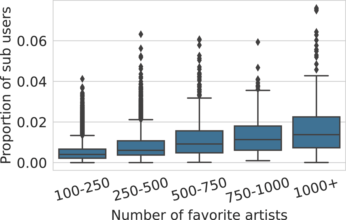
Figure 4
Distributions of how many users (in proportion of DL) have all their favorite artists included in those of a “power-user”, for various ranges of “power-user” collection size. For example, the likes of 1% of users are fully included on average in those of a user with 750–1000 favorite artists.

Figure 5
Proportion of users (from DL) whose favorite artists are included in the favorite artists of “power-users”. For example, 40% of users are included in users with more than 250 favorite artists.
Additionally, we computed Funiq_minsize on DS. Expectedly, streams allow a much higher identifiability than likes, as users like much fewer artists and songs than they stream (Figure 6). Extending the time period for retaining stream logs strongly increases identifiability: one month of stream logs is enough to identify 95% of the users.
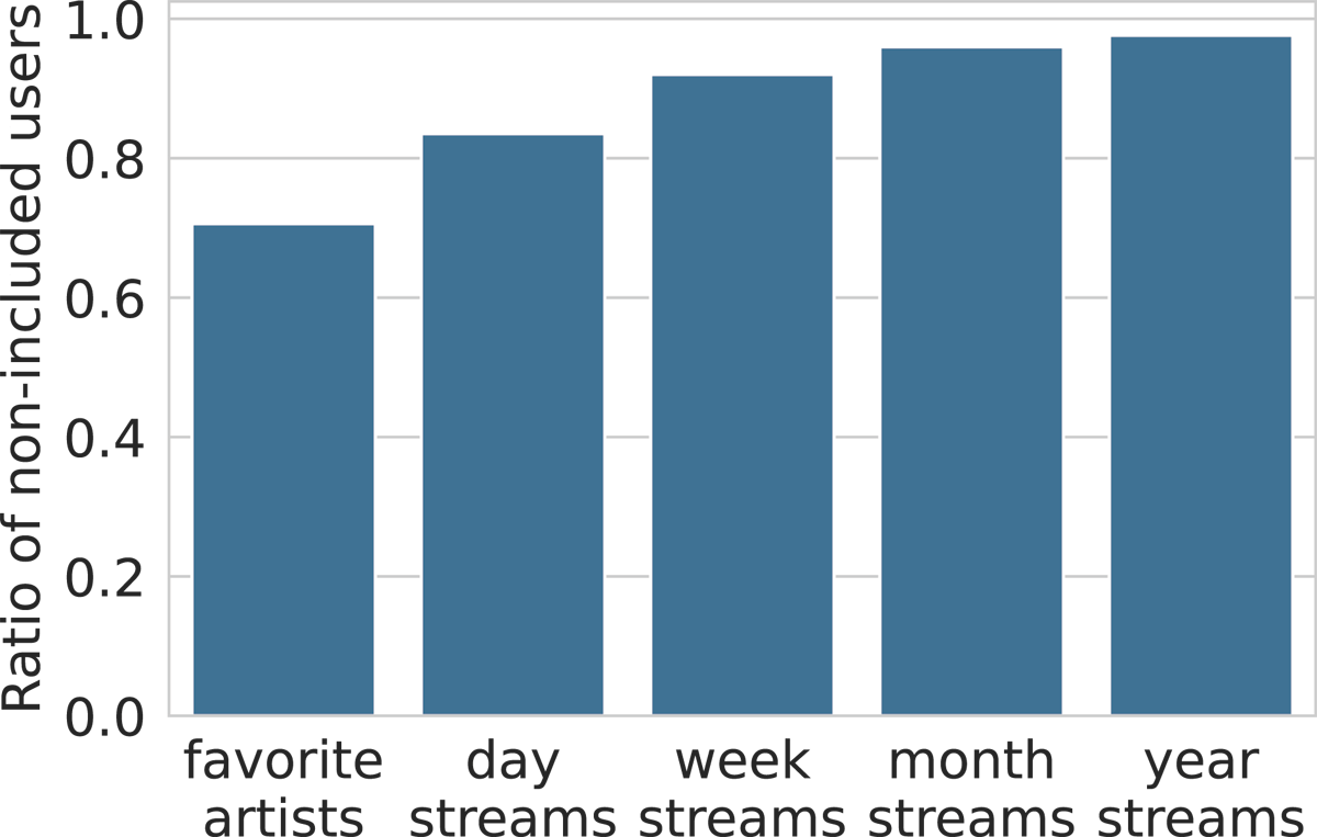
Figure 6
Ratio of users (from DS) identifiable through their liked and streamed artists, for different time periods. For example, 97% of the users are identifiable via their yearly streamed artists.
4.3.2 Fingerprint size
To answer RQ2, we first looked at the size of the assigned fingerprints. In DL, we find unique fingerprints of an average size of 6.7 artists and 3.6 songs by drawing random items (Figure 7). For songs, the maximum size fingerprint is huge (176 songs to discriminate one user). Indeed, the dataset contains a few users with huge collections of liked items, up to almost 105 favorite songs. The favorite items of such users are most likely to cover a lot of other users’ collections, which is why we would need this many items to discriminate them from others. However, considering the average and the median fingerprint size, which is 3 (for songs), we can assume that such a high fingerprint size is more of an exception than a rule.

Figure 7
Distributions of fingerprint sizes, computed with Funiq_rand and Funiq_minsize based on users’ favorite artists (DL).
With Funiq_minsize, we find unique fingerprints of an average size of 2.3 artists and 1.4 songs. Among 1M users, 45% of them are identifiable with only one song. Table 2 shows that the average size of fingerprints based on songs increases only slightly with the size of the dataset. It can thus be assumed that even though the number of identifiable users will decrease in a larger dataset (Table 2), the average size of unique minimum size fingerprints based on songs will remain around 1.5.
Table 2
Distributions of fingerprint sizes, computed with Funiq_rand and Funiq_minsize based on favorite artists and songs, for different numbers of users in the dataset.
| Artists | |||||||
| Sampling method | Number of users | Unique users (%) | Min F(u) size | Max F(u) size | Median F(u) size | Mean F(u) size | Standard deviation |
| Funiq_rand | 1000 | 87.3 | 1 | 13 | 2 | 2.4 | 1.4 |
| 10000 | 77.5 | 1 | 33 | 3 | 3.5 | 2.3 | |
| 100000 | 67.7 | 1 | 58 | 4 | 4.9 | 3.6 | |
| 871248 | 58.1 | 1 | 137 | 5 | 6.7 | 5.3 | |
| Funiq_minsize | 1000 | 87.3 | 1 | 4 | 1 | 1.3 | 0.5 |
| 10000 | 77.5 | 1 | 7 | 1 | 1.6 | 0.7 | |
| 100000 | 67.7 | 1 | 10 | 2 | 1.9 | 1.0 | |
| 871248 | 58.1 | 1 | 14 | 2 | 2.3 | 1.2 | |
| Songs | |||||||
| Funiq_rand | 1000 | 96.8 | 1 | 8 | 1.9 | 1.7 | 0.8 |
| 10000 | 94.4 | 1 | 33 | 2 | 2.2 | 1.2 | |
| 100000 | 92 | 1 | 98 | 3 | 2.9 | 1.7 | |
| 889017 | 89.9 | 1 | 176 | 3 | 3.6 | 2.4 | |
| Funiq_minsize | 1000 | 96.8 | 1 | 2 | 1 | 1.0 | 0.1 |
| 10000 | 94.4 | 1 | 5 | 1 | 1.1 | 0.3 | |
| 100000 | 92 | 1 | 8 | 1 | 1.3 | 0.5 | |
| 889017 | 89.9 | 1 | 194 | 1 | 1.4 | 1.1 | |
The fingerprints’ size based on favorite artists DS_favart (average 1.9, median 2) is comparable to one day of streams for the same users DS_day (average 1.8, median 2), and slightly decreases with larger time periods (average 1.4, median 1 for a year of streams DS_year).
4.3.3 Composition of the fingerprints
Another metric of interest to answer RQ2 is the fingerprints’ content. First, we compare the artists found in the fingerprints based on likes and streams, respectively DS_favart and DS_year. To this extent, we divide, for each user, the number of common artists by the total number of unique artists in both fingerprints. The found average ratio is around 1%, which means that there is no redundancy between the two kinds of fingerprints. Therefore, in a situation where anonymized streaming logs are shared, crossing this data with open access likes data should not lead to deanonymization, at least with the Funiq_minsize method.
To have a deeper understanding of what kind of music is more discriminative, we compare the popularity and genre distributions of the fingerprint items with the users’ favorite items in general (on DL). Unsurprisingly, the popularity of an artist or a song is an important indicator of whether or not it might be included in one’s fingerprint (Figure 8): the less popular the item, the more discriminative it is. As for the genres, the most popular ones, such as hip-hop, pop, rock and electronic music, seem to be underrepresented, while other, less popular genres, are overrepresented in the fingerprints (Figure 9).

Figure 8
Distribution of popularity among the artists in the fingerprints. We compare the distribution of popularity among users’ favorite artists, Funiq_rand fingerprints and Funiq_minsize fingerprints (DL).

Figure 9
Distribution of genres among the artists in the fingerprints. We compare the distribution of genres among users’ favorite artists, Funiq_rand fingerprints and Funiq_minsize fingerprints (DL).
If we consider musical taste through individuality and uniqueness, as Lahire (2008) did, we are then able to create fingerprints of musical taste. However, is individuality on its own a sufficient definition of taste, and do these unique fingerprints capture the essence of the users’ preferences?
5. Representative Musical Taste Fingerprints
The method we describe in the previous section can be used to distinguish users and to capture what makes their musical taste unique. In the process, it seems to have selected elements that do not necessarily reflect the overall distribution of their preferences.
In the previous section, we use the term fingerprint; in this section, we will keep using this concept, by analogy to the previous section, even though we are not looking to identify users anymore. Here, we consider a representative fingerprint as a set of items that summarize a user’s preferences. We use items, and not embeddings or other latent variables, as we want our fingerprint to be easily interpretable, and again, as a mirror with the previous section.
We propose to measure the representativeness of a fingerprint by means of a prediction task: i.e. given the subset of items selected, can we reconstruct the full set of a user’s liked items? We then present a fingerprinting method that allows us to build a representative fingerprint according to two defined evaluation methods. Finally, we compare it with the unique fingerprints computed in Section 4.
5.1 Problem definition
We formulate the problem in a way similar to recommendation: a subset F(u) is considered as representative of V(u) if there exists a method F⋆ such that ∀ u ∈ U, V(u) ≈ F⋆(F(u)),. In other words, we consider that a fingerprint is representative if a method that can recover the initial set of items from it exists. Building an F⋆ function is a ubiquitous task in recommender system research, where the problem is very similarly defined.
We chose to define F⋆ as a simple prediction function based on the nearest neighbor algorithm, computing the proximity between the artists using matrix factorisation (Koren et al., 2009). For favorite items, we start by building a sparse artist-user matrix M, where M[u,i]=1 if the user u has liked the artist i. For streams, M[u,i]=1 if the user u has streamed the artist i at least once during the given time span. We then compute a singular value decomposition (SVD), and use the first 128 dimensions of the SVD as our artists’ embeddings. The artists’ nearest neighbours are then computed based on the Euclidean distances between their embeddings.
Let N(i) be a list of i’s nearest neighbors ordered from the closest to the furthest. Let wi be a weight associated to each item i in a fingerprint F(u). This weight represents the number of items we need to recover from u. If all items in F(u) are equally important, then we want to recover the same number of items from each item in F(u): ∀ i ∈ F(U), wi = (|V(u)| – |F(u)|)/|F(u)|. For a user u, F⋆ returns a set of predicted items P(u) by simply taking, for each item i in F(u), the wi closest neighbors of i from the list of i’s 150 most similar artists.
5.2 Evaluation proxy
The representativeness score of a fingerprint is calculated based on how close the predicted items are to the user’s favorite items. We propose two methods to compare P(u) and V(u):
Item-wise. This evaluation is the most strict. The predicted items P(u) are compared exactly to the actual user’s favorite items (except the ones included in the fingerprint). The prediction accuracy for a user u is thus equal to |P(u) ∩ (V(u)|F(u))|/|P(u)|. This metric is widely used in recommender systems for offline evaluation tasks, where ground truth user-item interactions are available.
Genre-wise. Here, we compare if the predicted items follow similar distributions in terms of genre as the items from the user’s actual favorite items. The prediction score is thus simply the L1 distance between the distribution of genres in P(u) and the one in V(u).
Other metrics could also be used, based on the mainstreamness of the artists for example.
5.3 Experiments
5.3.1 A method to sample representative fingerprints
We propose a simple method, that we name Frep_kmedoid, to compute fingerprints that would be representative of the users’ preferences.
Considering that each artist is represented with an embedding of size 128 (computed in Section 5.1), the favorite artists of user u, V(u), are split into k clusters using the k-medoids algorithm. The medoids are then used as representative artists of each cluster to build the user’s fingerprint, and the weight w(i) associated to each artist i in the fingerprint is the size of the related cluster. We assume that the diversity of music genres in the users’ favorite artists varies from one user to another, thus the optimal k may not be the same for different users. In order to determine the optimal k for each user, we computed fingerprints with k going from 1 to 15% of |V(u)| (as we consider a fingerprint as concise information about the users’ preferences, we set maximum k limit to 20), then run the prediction task F⋆ on the obtained fingerprint. For each user, we retain the optimal k value that gave the highest prediction score with an item-to-item evaluation.
As a baseline, we use a method Frep_rand, which consists in randomly sampling k items in V(u) for a user u, with u’s optimal k value for Frep_kmedoid. Table 3 shows that the prediction scores for Frep_kmedoid fingerprints on liked items are indeed higher than with Frep_rand, both with item-to-item and genre-wise evaluation, and the score is higher for users with larger music collections. A better prediction accuracy is achieved with streaming data (Table 4) – for yearly streaming logs, we can restore almost 40% of the exact items through the fingerprints. Reaching an accuracy of 1 with an item-wise evaluation is not feasible within such a vast item space, and this level of precision is also uncommon in real-world recommendation systems. Based on the positive dynamics of the prediction accuracy on larger datasets, in the following, we will consider Frep_kmedoid as a method that aims to capture the essence of users’ musical taste.
Table 3
Item-wise and genre-wise prediction accuracy with Frep_kmedoid fingerprints and randomly sampled fingerprints of the same sizes on DS_favart.
| Frep_rand | Frep_kmedoid | ||||
| Evaluation | Number of favourite artists | Mean accuracy | Standard deviation | Mean accuracy | Standard deviation |
| Item-wise | <25 | 0.05 | 0.11 | 0.08 | 0.13 |
| 25–50 | 0.14 | 0.12 | 0.25 | 0.13 | |
| 50–75 | 0.16 | 0.12 | 0.28 | 0.12 | |
| 75–100 | 0.18 | 0.11 | 0.30 | 0.12 | |
| 100–150 | 0.21 | 0.12 | 0.32 | 0.12 | |
| >150 | 0.26 | 0.12 | 0.37 | 0.10 | |
| Genre-wise | <25 | 0.38 | 0.31 | 0.40 | 0.28 |
| 25–50 | 0.65 | 0.14 | 0.73 | 0.09 | |
| 50–75 | 0.70 | 0.13 | 0.78 | 0.08 | |
| 75–100 | 0.71 | 0.12 | 0.81 | 0.07 | |
| 100–150 | 0.77 | 0.10 | 0.83 | 0.08 | |
| >150 | 0.88 | 0.12 | 0.97 | 0.05 | |
Table 4
Prediction accuracy and optimal k with an item-to-item evaluation for Frep_kmedoid on favorite artists and streamed artists for different time periods (DS).
| Accuracy | Optimal k | |||
| Data sample | Mean | Standard deviation | Mean | Standard deviation |
| Favorite artists | 0.09 | 0.12 | 2.66 | 3.26 |
| Day streams | 0.07 | 0.11 | 1.86 | 1.67 |
| Week streams | 0.13 | 0.11 | 5.03 | 4.42 |
| Month streams | 0.26 | 0.13 | 8.82 | 5.70 |
| Year streams | 0.35 | 0.12 | 9.73 | 6.23 |
An interesting thing to notice is the optimal k size in different datasets: a smaller average fingerprint size is observed with favorite artists and single-day streams. The average size then grows with larger streaming time spans, and so does the standard deviation (Table 4). The average size can be easily connected to the amount of data to recover. Complementarily, the growing standard deviation can be explained by the heterogeneity of the users: on a one year span, some users will listen to a large variety of different genres, and some will stick to only a few, which is why the ideal fingerprint size might be very different from one user to another.
5.3.2 Uniqueness vs essence
To answer RQ3, we now want to confront our two sampling methods, Funiq_minsize and Frep_kmedoid.
First, we run both sampling methods on uniquely identifiable users DL_uniq, then run the prediction on both obtained fingerprints: the prediction accuracy from the unique fingerprints is lower (3% with item-to-item evaluation, 42% genre-wise) than the representative fingerprints (10% with item-to-item evaluation, 50% genre-wise) (Figure 10), meaning that the most discriminative items in the users’ libraries are not representative of their overall preferences.

Figure 10
Item-wise (top) and genre-wise (bottom) prediction accuracy with Funiq_minsize fingerprints and Frep_kmedoid fingerprints, performed on DL_uniq.
Second, we found that only 279 435 users remain identifiable from DL’s representative fingerprints, comparing to 507 037 in DL overall. Thus, extracting the essence of one’s musical library most likely leads to a loss of the information that makes them unique.
Trying to quantify the essence and the uniqueness of one’s musical taste seems to represent two diverging goals, which require distinct computation methods.
6. Discussion
6.1 Conclusion
Building on a large set of literature, we emphasize how preference elicitation encompasses several conflicting definitions. We propose to make two of them explicit, stressing constraints of uniqueness (respectively representativeness) as optimization goals adapted to distinction (respectively characterization) of an individual’s taste fingerprint. We show that these different constraints lead to diverging solutions which in turn suggests that scientific work addressing musical taste should probably reflect on their exact objectives and make their understanding of the term explicit.
We run our experiments using data from a major streaming platform, containing both explicitly liked content and streaming logs. In a first section of experiments, we show that in a sample of 1M active users, 90% can be identified by their favorite songs, and one or two songs is enough to identify 45% of the users. On another sample of 50K users, we also show that streaming logs are even more identifying, especially if collected for a long period of time – up to 97% of the users are identifiable via the artists they streamed for a year (RQ1).
However, the artists allowing to identify users are not the same when it comes to what they have liked or streamed. Also the more identifying items are expectedly the less popular ones, and by consequence, those from less popular genres (RQ2).
In a second section of experiments we propose a method to depict users’ preferences by creating representative subsets of users’ favorite items that we call fingerprints. This method can further be used in situations when concise information about the users’ preferences is needed: in recommendation systems, or scientific work that uses the concept of musical taste.
We show that the best items for identifying users are not the most representative of their preferences: using a prediction task, we can recover an average of 10% of the users’ favorite artists from the representative fingerprints against 3% from the unique fingerprints. Complementarily, only 279 435 users remain identifiable based on their representative fingerprints, against 507 037 in the initial set. It thus seems that the essence and uniqueness of musical taste are opposite concepts (RQ3).
6.2 Limitations
The experiments proposed in this work are nonetheless limited by the nature of the data used to conduct them. As we have emphasized, observable data are handy to collect at scale, but arguably they are non-perfect proxies of an individual’s true preferences. In particular, the information of explicit distaste is missing, though it appears to be a highly relevant indicator. An intuitive approach would be to leverage implicit feedback such as skips, but these are even noisier signals.
A more promising approach would be to build a richer, multi-modal dataset, containing both declared and observed data for a sufficient number of individuals. This will be the focus of our future work. Additionally, the evaluation of the fingerprinting methods could also be improved, in particular by means of an experiment involving the users themselves, for instance using an interface such as the one presented by Cura et al. (2022).
6.3 Addressing privacy issues
Unlike streaming logs, information about users’ likes is publicly accessible on the Deezer platform and most of their competitors, unless users specifically indicate their account as private. The fact that most users can be identified by their likes basically shows that a significant share of them are by default 1-anonymous Sweeney (2002), thus not anonymous. It reveals an important privacy issue – the usual practice of hashing the users’ IDs does not seem to be enough to anonymize a dataset. It can be especially compromising to share personal data, such as geolocation for example, combined with information about the users’ likes. Future work could be done to explore ways to aggregate or obfuscate such data in order to ensure k-anonymity, while keeping its expressiveness at the same time.
In the music information systems used on platforms, which must remain expressive for users, there is no category for describing music that would be both more precise than music genres (which are ill-defined categories) and more aggregated than the precise catalog items consumed by users: tracks, artists, and albums. Consequently, for lack of a better alternative, our results suggest that publicly available information about individuals’ music preferences should likely be aggregated at the level of music genres to strengthen anonymity (e.g. possibly defined as clusters of artists, whose size should be adjusted to ensure k-anonymity, with artist cluster sizes depending on k).
Notes
[1] www.deezer.com.
Acknowledgements
The authors thank the anonymous referees for their commitment to the peer-review process. Their valuable feedback and suggestions were of great help in shaping the final version of the paper.
Funding Information
This paper has been realized in the framework of the ‘RECORDS’ grant (ANR-2019-CE38-0013) funded by the ANR (French National Agency of Research).
Competing Interests
The authors have no competing interests to declare.
Author Contributions
KM, MM, TL and OB designed the study. KM analyzed the data and ran the experiments. KM, MM and TL drafted the manuscript. All authors wrote and approved the final version of the manuscript.