
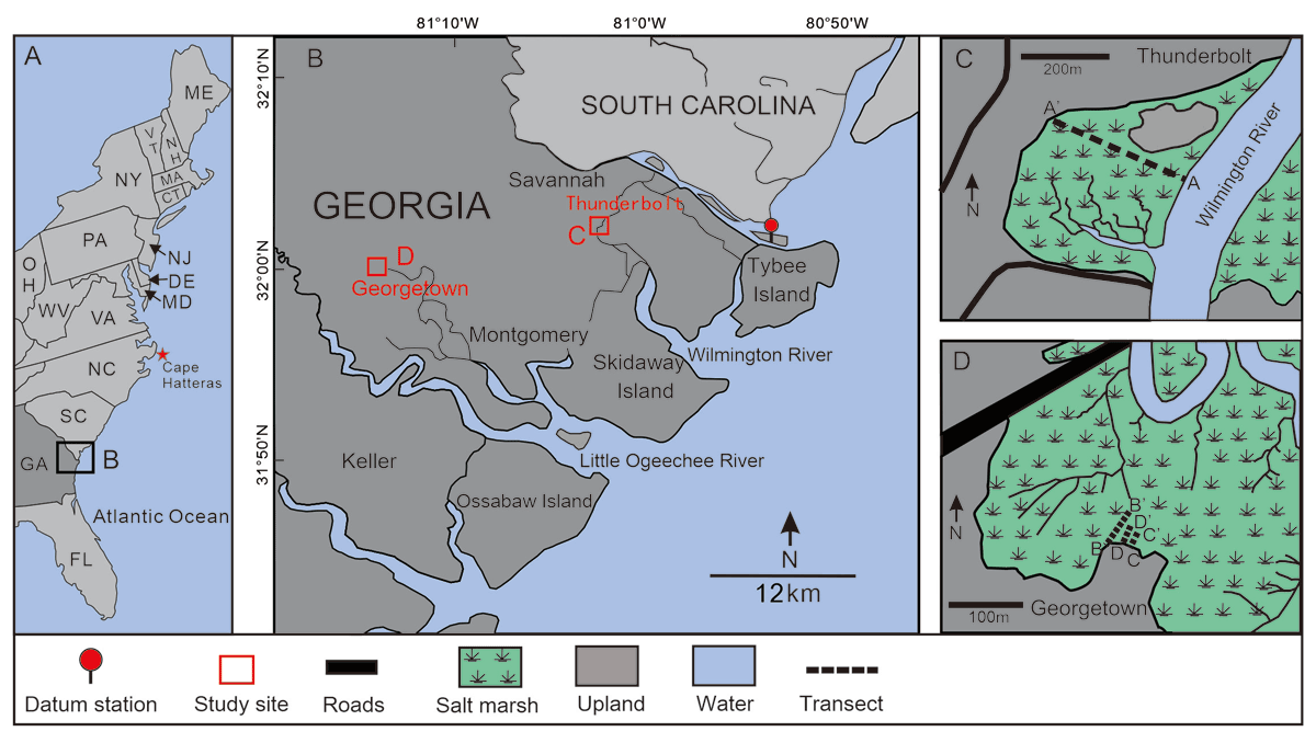
Figure 1
(A) U.S. Atlantic coast and location of study area in northern Georgia (B) Locations of two study sites at northern Georgia salt marshes. Tidal station is located at Fort Pulaski. Modern transect across the salt marshes at locations of (C) Thunderbolt and (D) Georgetown.
Table 1
Tidal datum’s relative to MTL for Fort Pulaski, Georgia.
| Datum | MLLW | MLW | MSL | MTL | NAVD88 | MHW | MHHW | HAT |
|---|---|---|---|---|---|---|---|---|
| Relative to MTL | –1.12 | –1.05 | 0.05 | 0.00 | 0.12 | 1.05 | 1.17 | 1.72 |
[i] Mean lower low water = MLLW, Mean low water = MLW, Mean sea level = MSL, Mean tidal water = MTL, North American Vertical Datum of 1988 = NAVD88, Mean high water = MHW, Mean Higher high water = MHHW, Highest Astronomical Tide = HAT.
Table 2
Sampling information for infaunal short cores.
| Core ID | Elevation (m MTL) | Salinity (‰) | Environment | Vegetation |
|---|---|---|---|---|
| TB-1-1 | –0.05 | 25 | Low marsh | Spartina alternaflora (50%), 50% bare clay, near riverbank |
| TB-1-22 | 1.16 | 20 | Low marsh margin | Spartina alternaflora (80%) |
| TB-1-24 | 1.19 | 0 | High marsh | Juncus roemerianus marsh. |
| GT-2-4 | 0.97 | 5 | High marsh | Spartina cynosuroides (25%), Juncus roemerianus (75%) |
| GT-2-5 | 0.91 | 10 | High marsh | Nearly 100% Juncus roemerianus |
| GT-2-10 | 0.69 | 0 | Mostly high marsh | Slight Spartina alternaflora, mostly Juncus roemerianus |
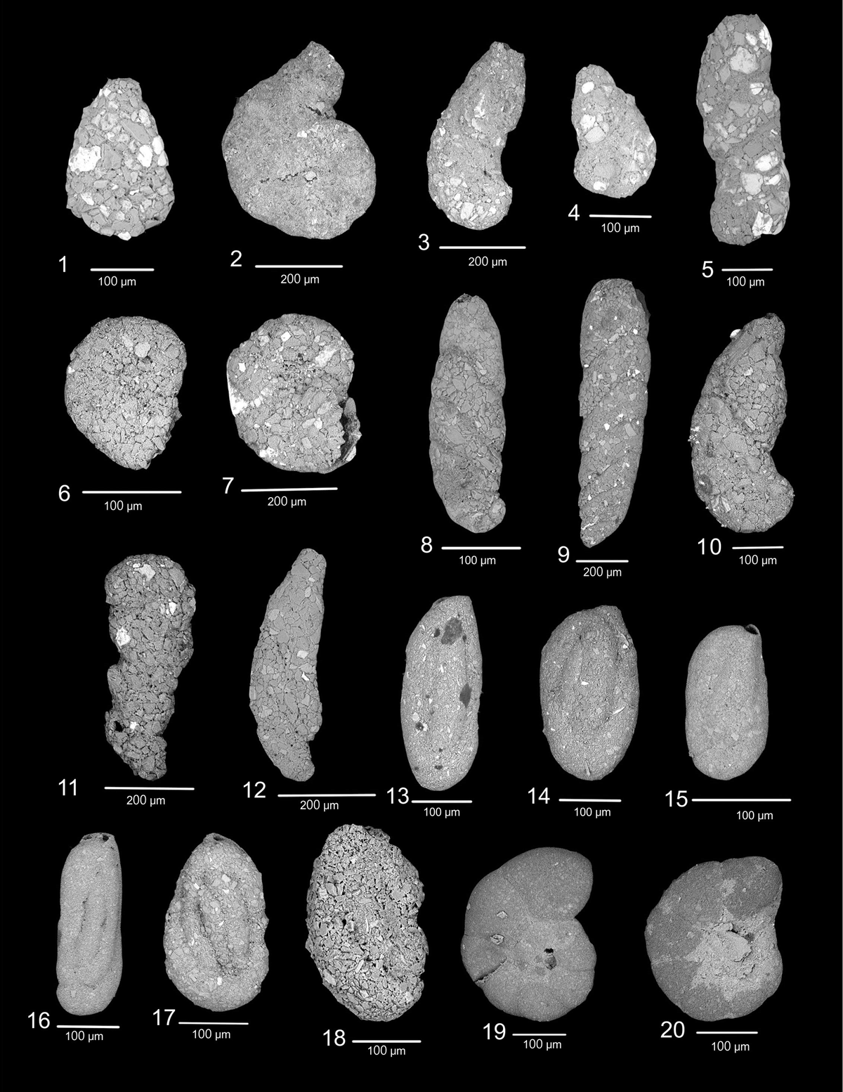
Plates 1
1, 2, 3, 4. Ammobaculites dilatatus (Cushman&Brönnimann, 1948) 5. Ammobaculites crassus (Warren, 1957) 6, 7. Ammobaculites sp. 8. Ammotium directum (Cushman & Brönnimann, 1948) 9. Ammotium salsum (Cushman & Brönnimann, 1948) 10, 11, 12. Ammotium spp. 13, 14. Miliammina fusca (Brady, 1870) 15, 16. Miliammina petila (Saunders, 1958) 17, 18. Miliammina spp. 19, 20. Balticammina pseudomacrescens (Brönnimann, Lutze & Whittaker, 1989).
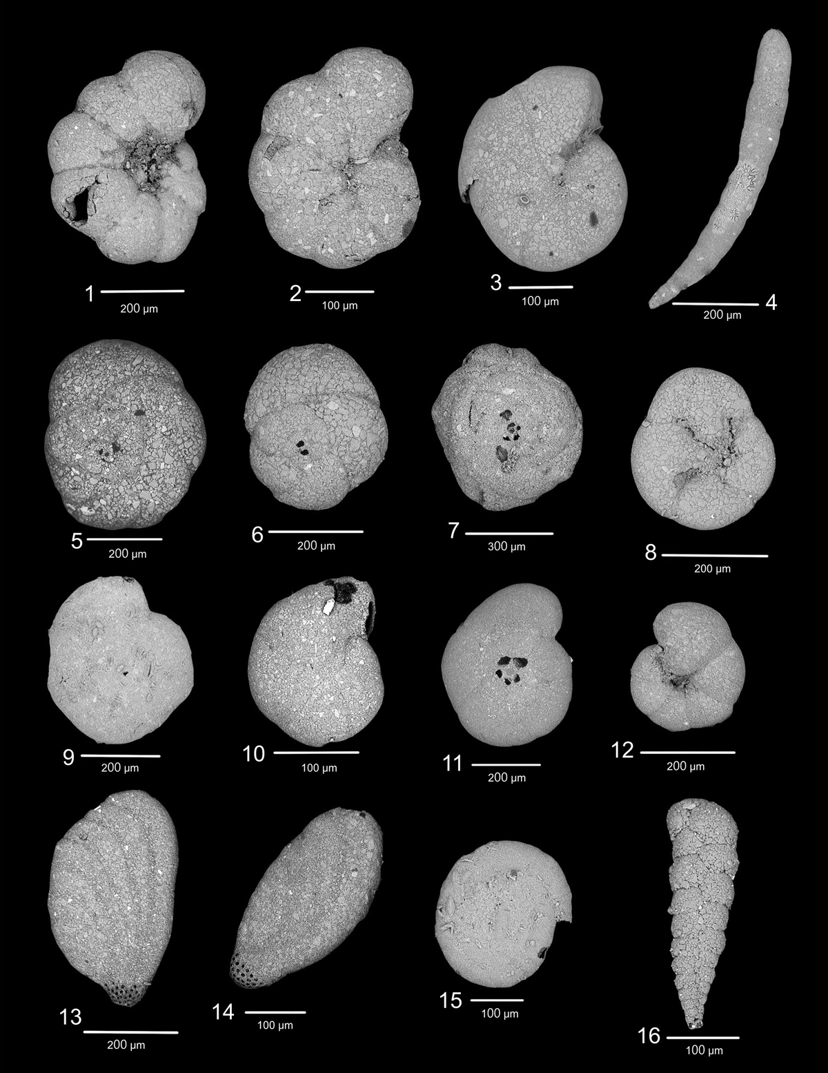
Plates 2
1, 2, 3 Haplophragmoides manilaensis (Andersen, 1952) 3. Haplophragmoides wilbert (Andersen, 1953) 4. Warrenita palustris (Warren, 1957) 5, 6, 7, 8. Tiphotrocha comprimata (Cushman&Brönnimann, 1948) 9,10. Arenoparrella mexicana (Kornfeld, 1931) 11, 12. Trochammina inflata (Montagu, 1808) 13, 14. Ammoastuta inepta (Cushman&McCulloch, 1939) 15. Ammodiscus sp. 16. Textularia earlandi (Parker, 1952).
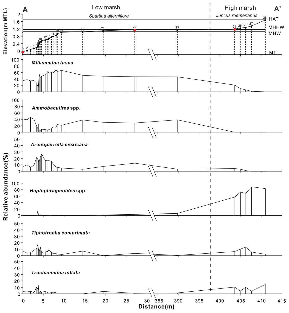
Figure 2
Modern distribution of the relative percentage of dead foraminifera plotted by distance for transect A-A’ at Thunderbolt. Vegetation zone and tide levels with respect to local mean tidal level (MTL) are shown. Transect locations are shown in Figure 1C. Only the taxa that are most important in defining ecological zones are presented. The dashed line divides the low and high marsh based on foraminifera. Red circles represent locations of infaunal cores.
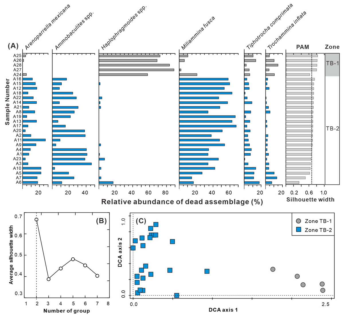
Figure 3
(A) Composition of the foraminiferal distribution and average silhouette width determined by partitioning around medoids (PAM) from Thunderbolt. The dashed line indicates average silhouette width of two groups. Shaded zone emphasize two different groups, each group is labeled (e.g.TB-1). (B) Average silhouette width estimated by PAM for the foraminiferal dataset indicating two groups (dashed vertical line) was appropriate. (C) DCA plot of samples from Thunderbolt salt marsh on the first two discriminant axes.
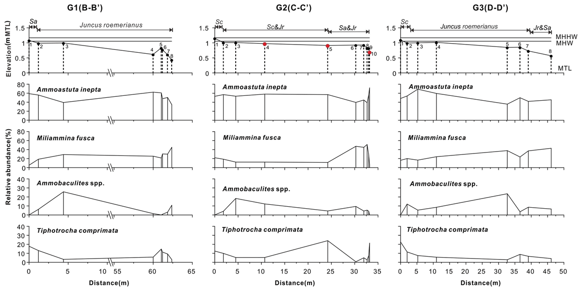
Figure 4
Modern distribution of the relative percentage of dead foraminifera plotted by distance for transects at Georgetown. Vegetation zones and tide levels with respect to local mean tidal level (MTL) are shown. Transect locations are shown in Figure 1D, G1 is for transect B-B’, G2 is for transect C-C’, and G3 is for D-D’. Only the taxa that are most important in defining ecological zones are presented. Red circles represent the locations of infaunal cores. Sa = Spartina alterniflora, Sc = Spartina cynosuroides, Jr = Juncus roemerianus.
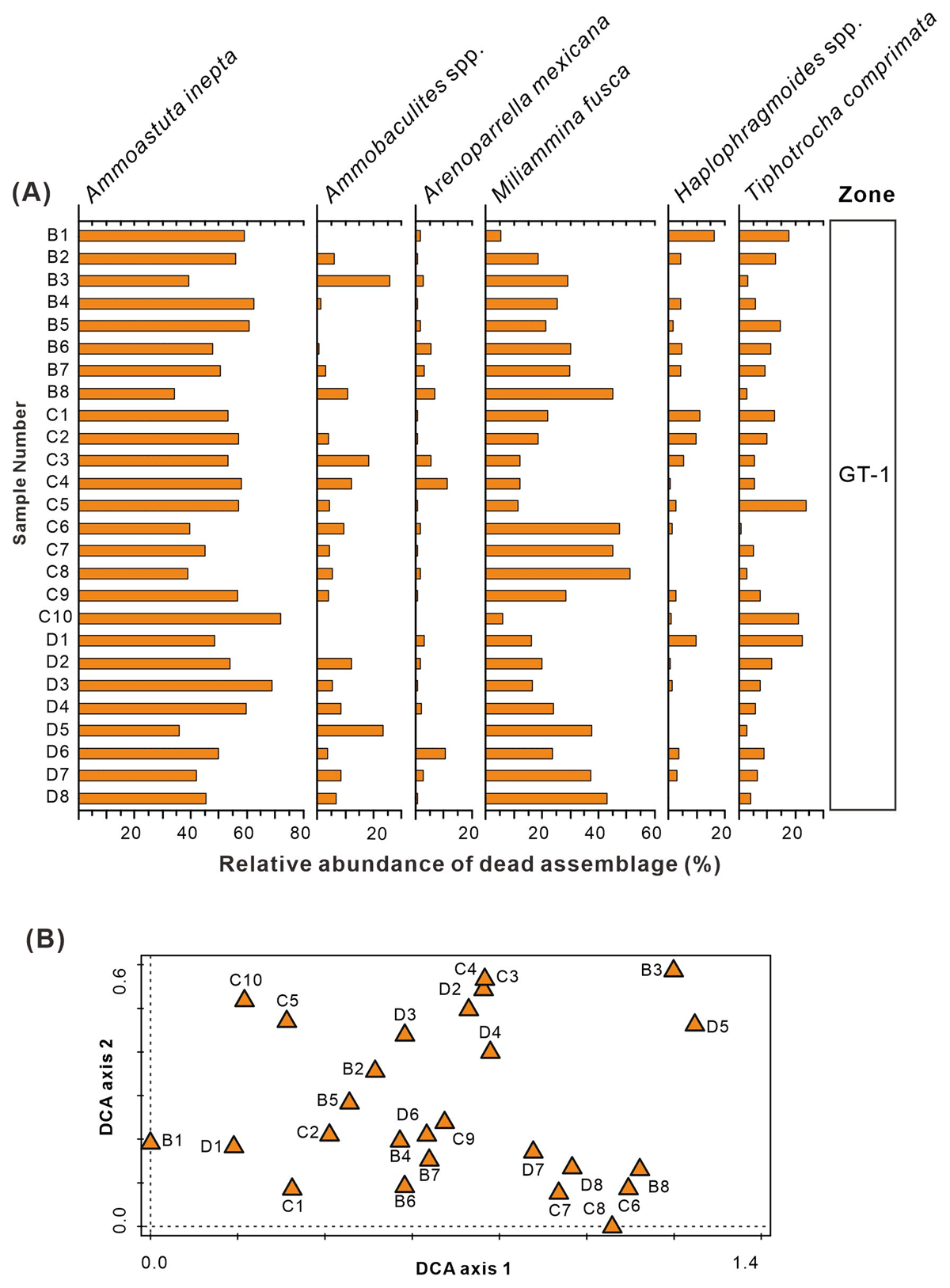
Figure 5
(A) Composition of the foraminiferal clusters identified by partitioning around medoids (PAM) from Georgetown. Only one group was recognized. (B) DCA plot of samples from Georgetown salt marsh on the first two discriminant axes.
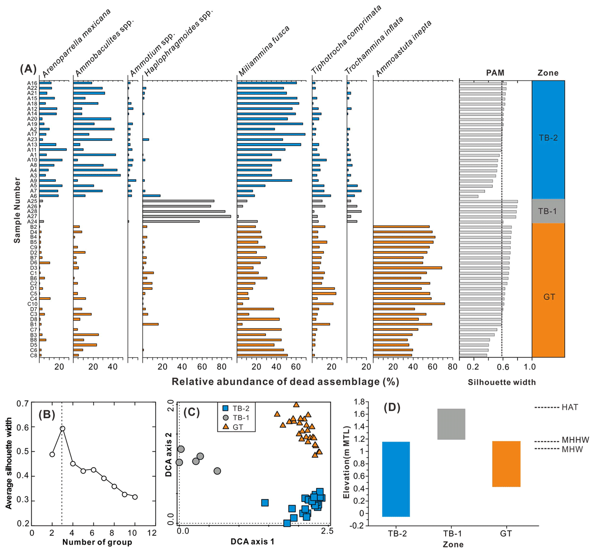
Figure 6
(A) Composition of the foraminiferal distribution and average silhouette width determined by partitioning around medoids (PAM) from combined dataset of Thunderbolt and Georgetown. The shaded zone emphasizes different groups, each group is labeled (e.g. TB-1). (B) Average silhouette width estimated by PAM for the combined foraminiferal dataset indicating three groups (dashed vertical line) was appropriate. (C) DCA plot of samples from both marshes on the first two discriminant axes. Samples are divided into the three zones. (D) Boxplots of faunal zones plotted by elevation (respect to MTL) with tidal levels superimposed.
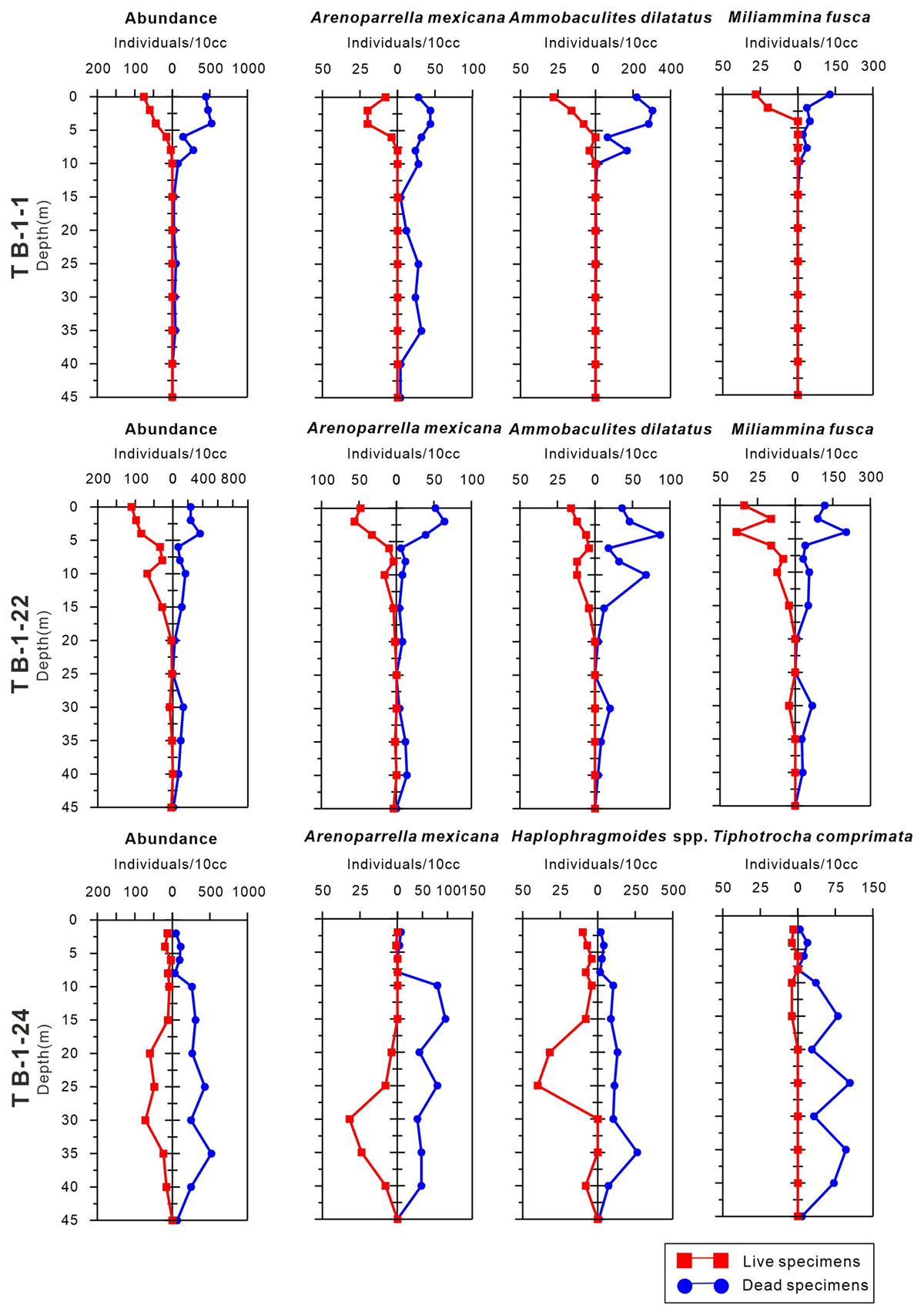
Figure 7
The live and dead assemblage density and numbers for most representative species plotted by core depth from Thunderbolt marsh. Core TB-1-1 (Elevation: –0.05 m MTL), TB-1-22 (Elevation: 1.16 m MTL), TB-1-24 (Elevation: 1.19 m MTL).
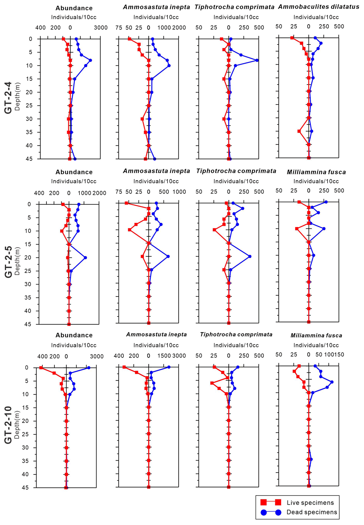
Figure 8
The live and dead assemblage density and numbers for most representative species plotted by core depth from Georgetown marsh. Core GT-2-4 (Elevation: 0.97 m MTL), Core GT-2-5 (Elevation: 0.91 m MTL), Core GT-2-10 (Elevation: 0.69 m MTL).