
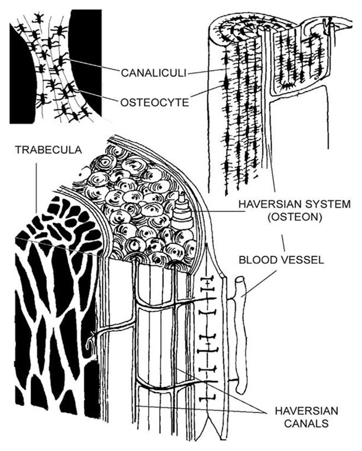
Figure 1
Sketch of the microscopic components of bone showing Haversian systems and osteocytes. Reproduced from Smit, Burger, and Huyghe 2002 p. 2022, with permissions from John Wiley and Sons under licence 5297961008734.
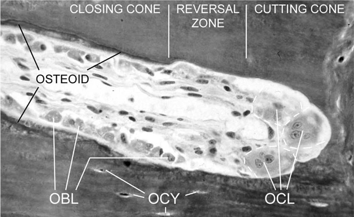
Figure 2
An example of an active Bone Multicellular Unit (BMU) showing osteoclasts (OCL), osteoblasts (OBL), and osteocytes (OCY). Image is not to scale, but the width of the BMU would be approximately 200 μm. Reproduced from Smit, Burger, and Huyghe 2002 p. 2024, with permissions from John Wiley and Sons under licence 5297961008734.
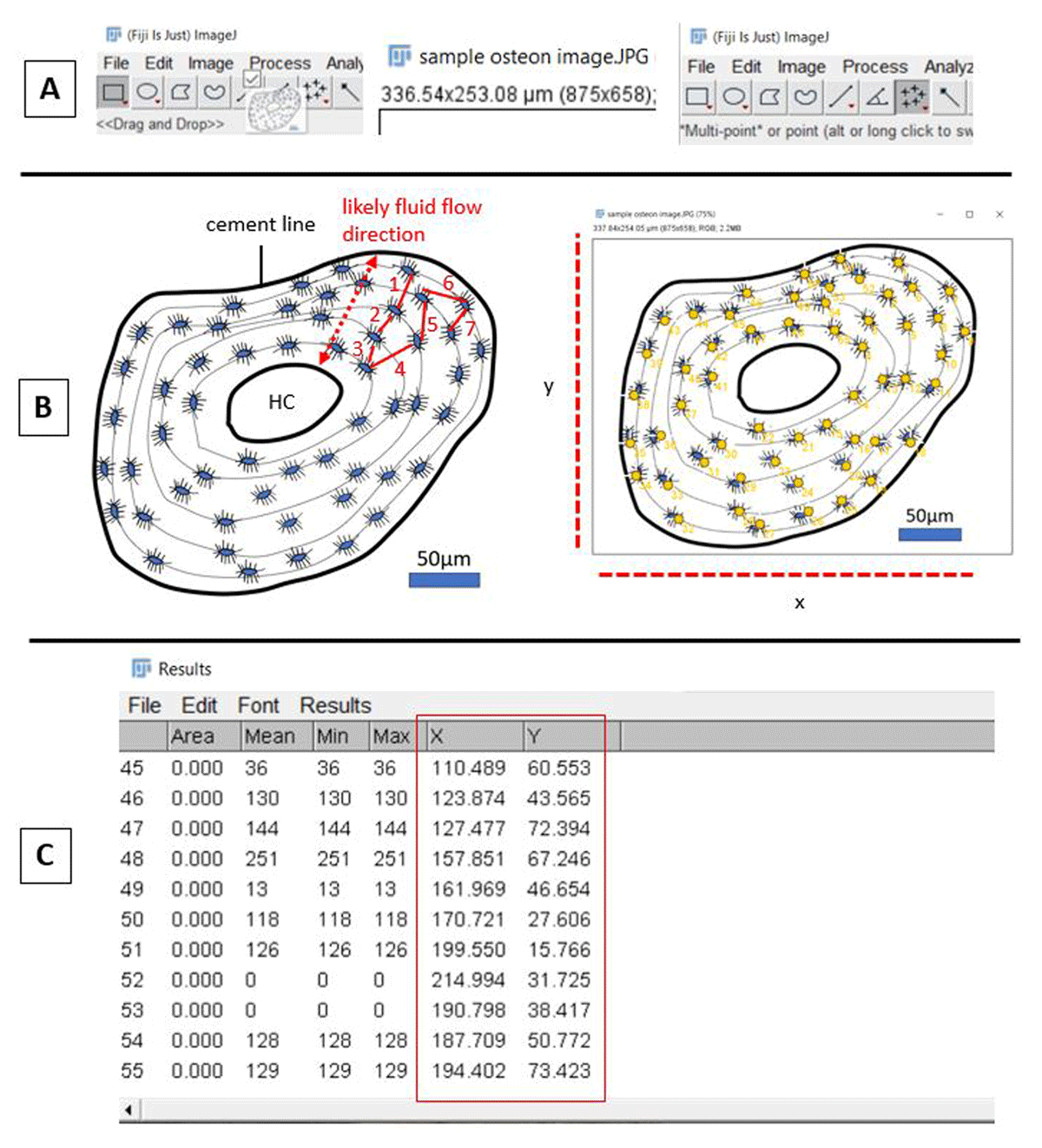
Figure 3
Series of initial steps of point counting in ImageJ/FIJI. A: importing of image (HC: Haversian canal), setting the scale, and selecting the “Multi-Point” tool. B: outline of secondary osteon diagram with osteocyte lacunae prior to (left), and after (right), counting of the lacunae. C: ImageJ/FIJI data window showing XY coordinates for each point (red box, left).
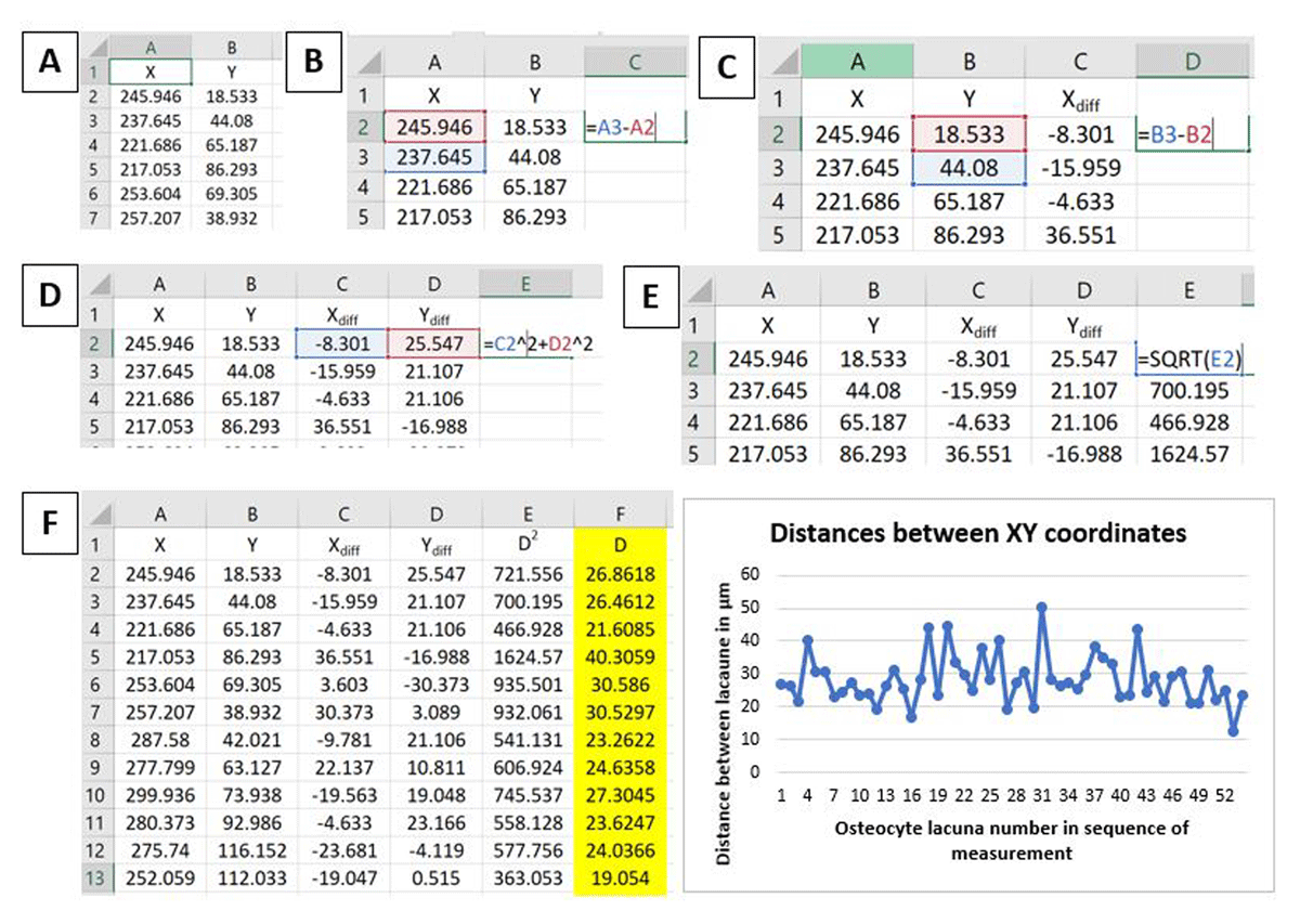
Figure 4
Screenshots of successive steps in XY distance coordinate calculations in Microsoft Excel. A: XY coordinates from the ImageJ/FIJI results output, B–C: calculating differences between successive X and Y coordinates, D: calculating the squared distance (D2) between XY differences, E: calculating the square root of D2, F: final distance values of XY coordinates (D) in μm (highlighted in yellow), which can be quickly visualised using a simple line graph.
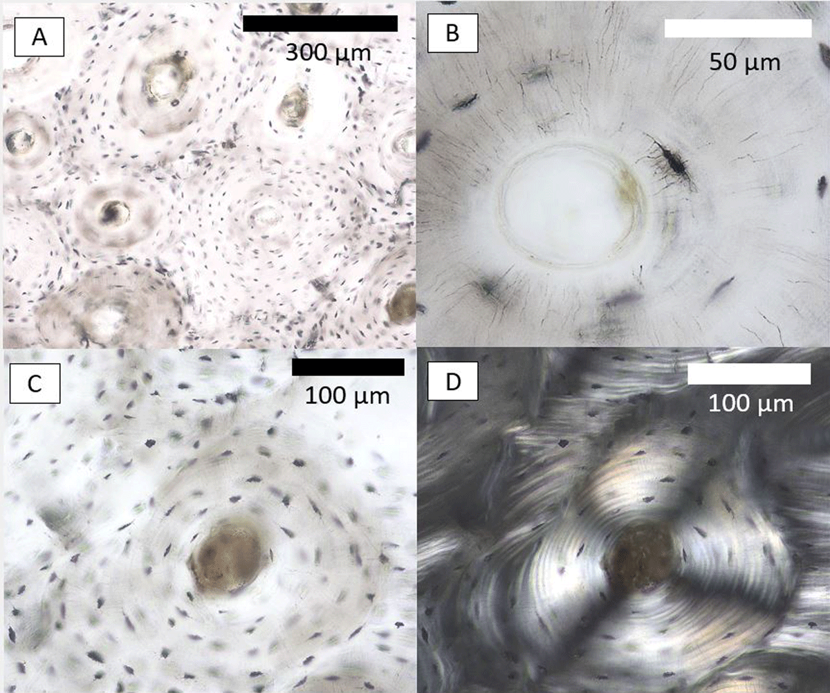
Figure 5
Cortical bone histology images in a sample from a Medieval English male (ID: NGB89SK2, St. Gregory’s Priory and Cemetery collection, University of Kent, UK) taken from the anterior midshaft. Image A shows a cluster of secondary osteons with a range of osteocyte lacunae preservation. Image B shows a closeup of an osteocyte lacuna as an example of good preservation in the secondary osteon selected for our replication analysis. Images C and D show the secondary osteon under polarised transmitted (C) and linearly polarised light (D).
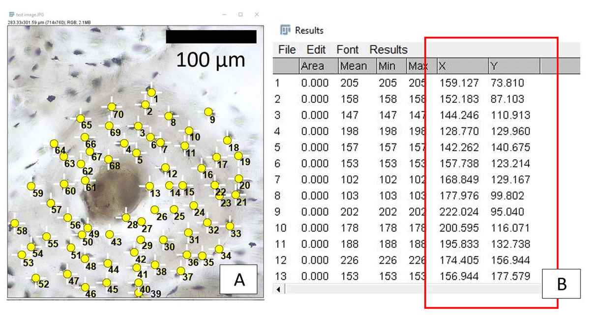
Figure 6
Screenshots of image analysis steps replicating our XY coordinate calculation protocol. A: secondary osteon with osteocyte lacunae (yellow dots). B: raw data output window in ImageJ/FIJI showing resulting XY coordinates (red rectangle).
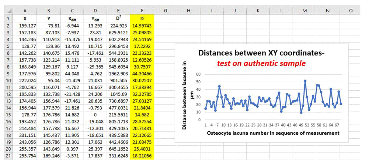
Figure 7
Screenshot of final calculations of distances between XY coordinates yielded using the Medieval English histology sample. Column F, highlighted in yellow, shows the D values in μm. The line graph illustrates variation in D values from across the entire secondary osteon.
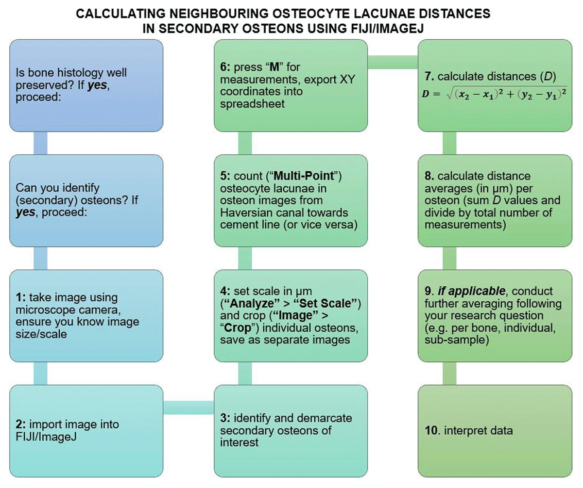
Figure 8
Flowchart summarising the steps of the protocol covered in our study. Please refer to text for more detail.