
1. Introduction
Quantitative analysis of histology images (histomorphometry) is a gold standard in various biological disciplines that collect data about tissue cells and other microscopic structures (e.g., Erben & Glösmann 2019; Revell 1983; O’Driscoll et al. 1999; Villa & Lynnerup 2010). Where there is good preservation, thin section histology can be studied in bones that derive from palaeontological and archaeological contexts to reconstruct remodelling processes (bone resorption and deposition) that occur throughout an animal’s lifespan and respond to internal and environmental stimuli (e.g., Bromage et al. 2009; Cook, Molto & Anderson 1998; Crowder & Stout 2011; de Buffrénil et al. 2021; Miszkiewicz 2015; Sawada et al. 2004; Stout & Stanley 1991). Questions of significance to human evolution, for example, were previously addressed by directly measuring bone histology characteristics to find similar rates of remodelling in femora of Holocene (15th–16th centuries Pecos Pueblo humans) and Pleistocene (‘Late Archaic’ Homo from Broken Hill, Shanidar, Tabun; and ‘Early Modern’ Skhul) hominins (Abbott, Trinkaus & Burr 1996; Streeter et al. 2010). Improving our understanding of human life history was previously achieved by histologically sampling juvenile chimpanzee (Pan troglodytes) femur, tibia, and fibula and showing that their age-related development was similar to juvenile humans (Mulhern & Ubelaker 2003). Holocene human bone histology analyses, using archaeological, forensic, and clinical sources, have gathered significant data on a series of topics such as age (e.g., Maggio & Franklin 2019), disease (see Schultz 2001), or biomechanics (e.g., Schlecht et al. 2012). Non-hominin examples include examination of rib histology in dwarfed insular Candiacervus deer from Pleistocene Crete, in which remodelling was found to be similar to that of larger mainland deer counterparts (Miszkiewicz & van der Geer 2022). Lifestyle-related differences in histological characteristics of the tibia between free-ranging wild boar (Sus scrofa) and domestic pigs (S. domesticus) helped us understand the impact of domestication on animal skeletal adaptation (Mainland, Schutkowski & Thomson 2007). These examples demonstrate the potential thin section histology has for advancing Quaternary palaeobiology research.
One specific technical approach in bone histology is quantifying geometric and density properties of secondary/Haversian bone tissue seen microscopically in thin sections taken in a transverse plane (Stout & Crowder 2012) (Figure 1). The histological appearance of Haversian bone reflects the activity of Bone Multicellular Units (BMUs) which are three-dimensional (3D) cell structures that execute bone remodelling in live bone by ‘digging’ longitudinal tunnels as bone is resorbed and deposited (Figure 2) (Lassen et al. 2017; Maggiano et al. 2016; Sims & Martin 2014). Once quantified, cortical bone histology data can be studied at an individual or large sample level representing past populations (e.g., Chan, Crowder & Rogers 2007; Stout & Lueck 1995; Miszkiewicz et al. 2020). All bone biologists who undertake histomorphometry are expected to follow recommended guidelines for unified nomenclature and techniques used in calculating parameters of bone remodelling (Dempster et al. 2013). Working with Haversian tissue, the relevant quantifiable histology variables include the area, diameter, density, and circumference of structures such as secondary osteons, Haversian canals, and osteocyte(s)/lacunae (osteocytes do not always preserve in post-mortem bone, so osteocyte lacunae indicate where the osteocytes had resided) (Bromage et al. 2009; Crowder & Stout 2011; Hunter & Agnew 2016; Stout, Cole & Agnew 2019). The densities of secondary osteons or osteocyte lacunae are typically calculated by summing up the total counts seen in a specified field of view or a selected region of interest (ROI), and then dividing the raw count by the area examined (Crowder et al. 2022; Crowder & Stout 2011; Drew, Mahoney & Miszkiewicz 2021). This counting approach is known as the ‘point count’ technique (Stout & Stanley 1991). Secondary osteon density, referred to as osteon population density (OPD), data reflect the amount of remodelled bone per area (Frost 1987), whereas osteocyte density reflects osteoblast-osteocyte conversion (Bromage et al. 2016).
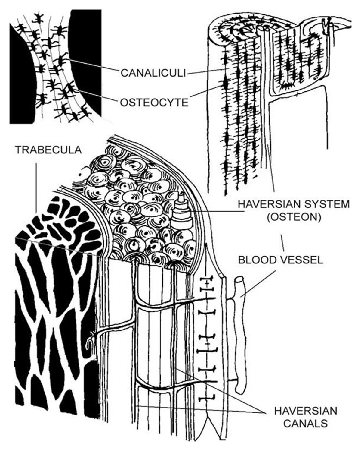
Figure 1
Sketch of the microscopic components of bone showing Haversian systems and osteocytes. Reproduced from Smit, Burger, and Huyghe 2002 p. 2022, with permissions from John Wiley and Sons under licence 5297961008734.
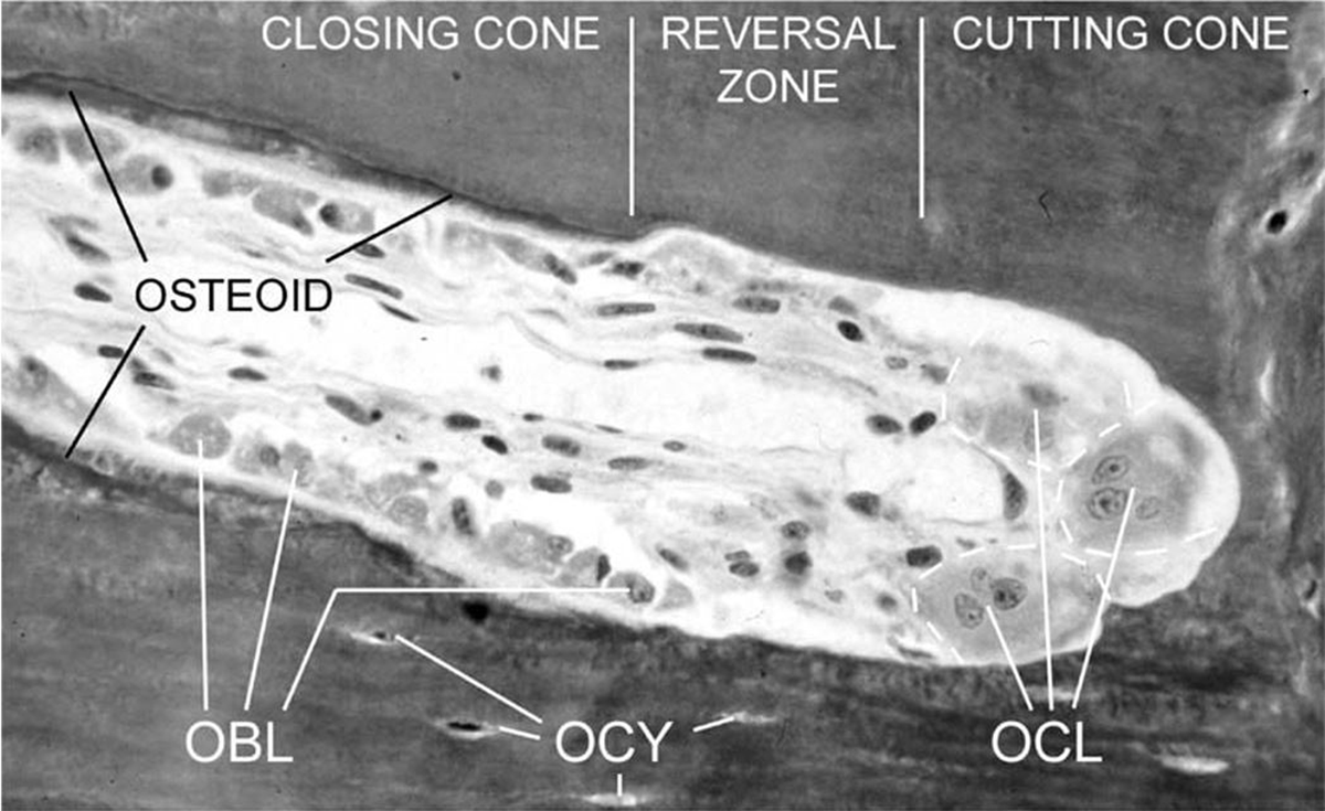
Figure 2
An example of an active Bone Multicellular Unit (BMU) showing osteoclasts (OCL), osteoblasts (OBL), and osteocytes (OCY). Image is not to scale, but the width of the BMU would be approximately 200 μm. Reproduced from Smit, Burger, and Huyghe 2002 p. 2024, with permissions from John Wiley and Sons under licence 5297961008734.
While these densities have been reported by multiple studies investigating topics that have ranged from biomechanics (Drew, Mahoney & Miszkiewicz 2021), diet (Paine & Brenton 2006), to human evolution (Sawada et al. 2004), a notable gap in analyses is that the proximities of individual counted points are not considered. This is interesting because biologists regularly consider dispersal or proximity analysis when analysing points against a specified area to assess the randomness, clustering, or migration of cells (Cruz et al. 2005; Fernández, Lysakowski & Goldberg 1995; Gorelik & Gautreau 2014; Wang et al. 2021). Only a handful of palaeontological, bioarchaeological, or anthropological studies have considered spatial distribution relationships within bone histology sections. This has included Rose et al. (2012), and Gocha and Agnew (2016), who brought to light the value of applying Geographic Information Systems (GIS) software in understanding osteon population dispersal across complete human metatarsal and femoral bone cross-section shafts, respectively. Further, Miszkiewicz et al. (2020) applied GIS to measure distances between neighbouring Haversian canals across thin sections from the femoral midshaft in an archaeological specimen, spatially mapping cortical bone porosity. Because GIS can require substantial training, an alternative, commonly used, user friendly, and self-intuitive image analysis software is the open access ImageJ, part of the FIJI package (Schindelin et al. 2015). In this paper, we highlight that ImageJ/FIJI also registers Cartesian (XY) coordinates alongside point counts and can be used to efficiently calculate path distances between neighbouring histology structures. We focus on hypothetical osteocyte lacunae in a sketched diagram, supply a manual protocol based on established mathematics for the path distance calculations, and then replicate it on a secondary osteon image from an archaeological (dated to Medieval England) human femur. While we use an archaeological human sample, this protocol can be applied to a range of vertebrates that experience Haversian remodelling, including mammals, birds, and some reptiles (Currey 2006; Hillier & Bell 2007; Mitchell et al. 2017; Padian, Werning & Horner 2016), as long as secondary osteons, with preserved osteocyte lacunae, can be clearly seen in their bone histology when analysed microscopically.
2. Methods: XY coordinates in imageJ/FIJI
2.1. The protocol and application to a hypothetical sample
ImageJ/FIJI can be freely downloaded from the dedicated website (https://imagej.net/software/fiji/). The preparation of bone histology slides will not be covered here. An image with a known scale captured using a dedicated microscope camera is needed to apply the protocol we discuss. We note ImageJ/FIJI provides macros and plug-ins that calculate various other aspects of XY coordinates (e.g., distance from centroid), but these require coding and script amendments. Distances between selected points can also be measured manually one by one using the “Straight line” tool of ImageJ/FIJI, but this approach takes more time than the presented XY coordinate analysis and has to be conducted in addition to point counting. We provide a manual guide for path distance calculations from the XY coordinate data recorded at the same time as point counts which is straightforward and efficient in its application.
The first step (Figure 3A) is to open ImageJ/FIJI (we used vol. 153o), import the image of interest, and set the appropriate scale (“Analyze” > “Set scale”). The counts of the osteocyte lacunae can be completed using the “Multi-point” function selected form the ImageJ/FIJI toolbar. For the distances to be most meaningful biologically, the sequence of counts made would ideally be either conducted starting at the Haversian canal and continuing outwards (towards the cement line), or vice versa (Figure 3B). That is because canaliculi, which connect successive osteocytes within a secondary osteon, are largely arranged radially so as to maximise fluid flow (van Tol et al. 2020). By pressing “M”, the measurements can be obtained. A “Results” window will appear where the following measurements are recorded: “Area”, “Mean”, “Min”, “Max”, “X”, “Y” (Figure 3C). The “X” and “Y” are the coordinate values that can be used to understand the proximity of these points. The output from the “Results” window can be saved as an Excel spreadsheet, or the XY coordinates can be copied and pasted into a new spreadsheet.
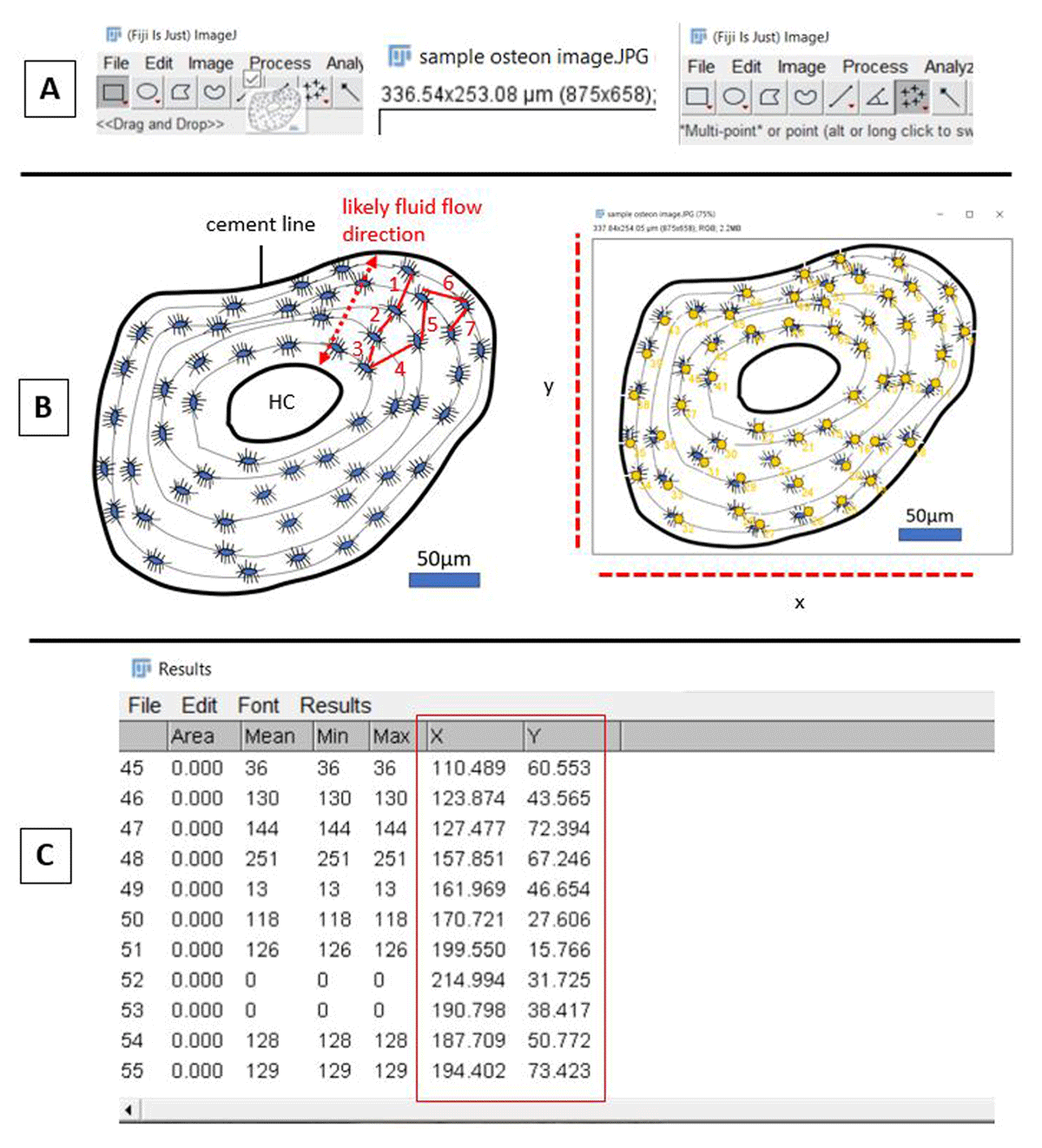
Figure 3
Series of initial steps of point counting in ImageJ/FIJI. A: importing of image (HC: Haversian canal), setting the scale, and selecting the “Multi-Point” tool. B: outline of secondary osteon diagram with osteocyte lacunae prior to (left), and after (right), counting of the lacunae. C: ImageJ/FIJI data window showing XY coordinates for each point (red box, left).
The next step is to calculate the 2D distance between XY coordinates, following the path of counting, using the formula (derived from the Pythagorean theorem) (Figure 4).
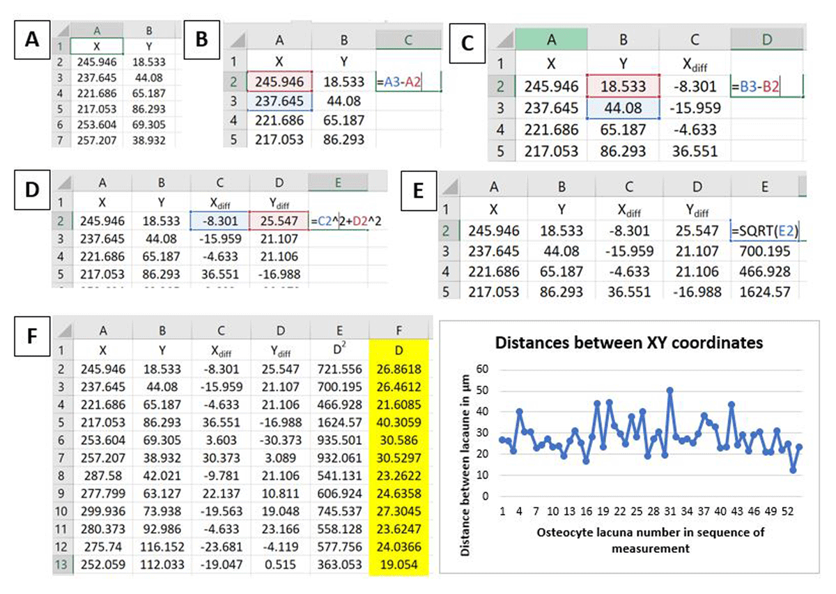
Figure 4
Screenshots of successive steps in XY distance coordinate calculations in Microsoft Excel. A: XY coordinates from the ImageJ/FIJI results output, B–C: calculating differences between successive X and Y coordinates, D: calculating the squared distance (D2) between XY differences, E: calculating the square root of D2, F: final distance values of XY coordinates (D) in μm (highlighted in yellow), which can be quickly visualised using a simple line graph.
In the same or a new spreadsheet, new columns aligned next to each other can be created and named: Xdiff (this will be the difference between successive X coordinates), Ydiff (this will be the difference between successive Y coordinates), D2 (squared distance between Xdiff and Ydiff), D (square root of D2).
The difference between successive X and successive Y coordinates is then calculated individually (i.e., per axis). This can be achieved in Microsoft Excel by typing in “=cell with raw X value-preceding cell with raw X value” – the example in Figure 4 would be “=A3-A2”. This then can be repeated on the Y coordinates. The last cell should not be considered because it does not have a successive coordinate. The cell function can be dragged down the entire column.
D2, defined through the formula: D2 = Xdiff2 + Ydiff2, is then calculated. This can be achieved in Excel by typing “=cell with Xdiff^2+cell with Ydiff^2”. The example shown in Figure 4 would be “=C2^2+D2^2”. The cell function can be dragged down the entire column.
Finally, the square root of D2 is calculated which can be done in Excel by typing “=SQRT(cell with D2 value). In Figure 4, the example would be “=SQRT(E2)”. The cell function can be dragged down the entire column.
Raw data resulting from this hypothetical image analysis can be found in our Supplemental File. The resulting D values are the distances in the unit appropriate to the image between the XY coordinates registered along the pathway of counting. They can be analysed across a whole osteon, summarised as averages per osteon, a full image, individual, larger sample – whatever the desired level of analysis as per one’s research question. In the presented example, the average distance across this one hypothetical secondary osteon was 28.25 μm (see Supplemental File).
2.2. Replication on an authentic sample
To validate this short protocol, we applied it step-by-step to a real case—using a cortical bone histology image showing a well-preserved secondary osteon in the femur of a Medieval English individual (ID: NGB89SK2). The thin section is a 100 μm-thick slice of midshaft cortex extracted from the anterior aspect of the femur. This individual was estimated to be a middle-aged (35–50 years old) male (Miszkiewicz, 2014), and the sample is part of a larger collection of thin sections representing a Medieval English human osteological assemblage curated at the University of Kent, UK. These thin sections had been prepared following standard histology methods applied to archaeological human remains (Miszkiewicz, 2014). A full ethics board review was not required as this is an archaeological collection, but a local (School of Anthropology and Conservation) ethics application form and check list was filed on 11 November 2010 and approved by the 2010 Ethics Advisory Group at the University of Kent, UK. In addition to curatorial permissions, all analyses on these sections follow codes of ethics and good practice as stipulated by the international biological anthropology bodies (British Association for Biological Anthropology and Osteoarchaeology; American Association of Biological Anthropologists). The anterior femur sample presented here was also previously included in research by Drew, Mahoney and Miszkiewicz (2021), Miszkiewicz and Mahoney (2012), and Miszkiewicz (2014). The XY coordinate distance data are calculated here for the first time.
Using an Olympus BX60 high powered microscope equipped with a MIchrome 5 Pro SS-936 camera and operated using Capture v2.1 software, one secondary osteon showing clear cement lines (Figure 5A) and well-preserved osteocyte lacunae (Figure 5B) was selected from intra-cortical bone. It was viewed under linearly polarised light to check good preservation, i.e., ensuring that individual concentric lamellar rings could be seen clearly (Figure 5C, D).
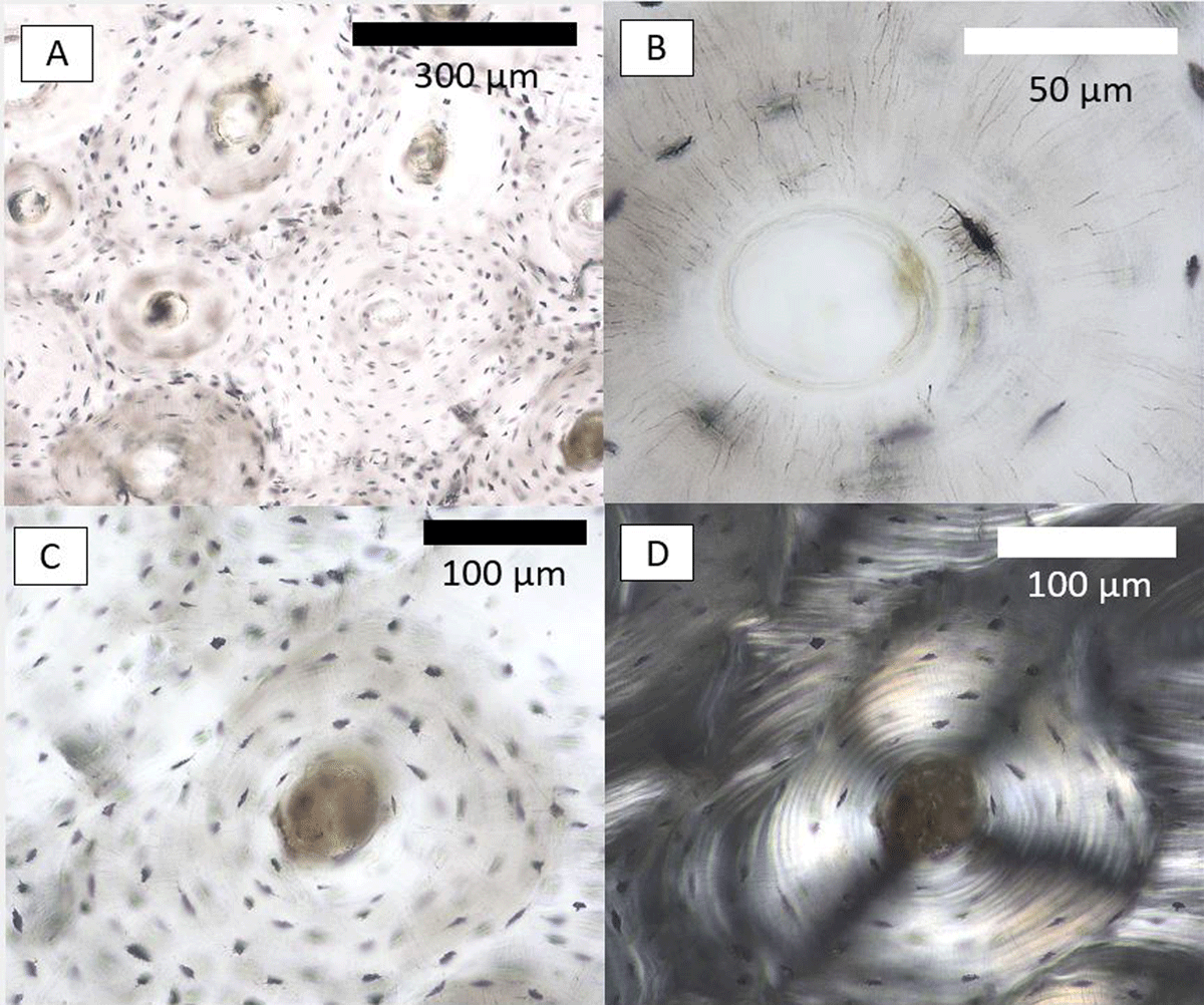
Figure 5
Cortical bone histology images in a sample from a Medieval English male (ID: NGB89SK2, St. Gregory’s Priory and Cemetery collection, University of Kent, UK) taken from the anterior midshaft. Image A shows a cluster of secondary osteons with a range of osteocyte lacunae preservation. Image B shows a closeup of an osteocyte lacuna as an example of good preservation in the secondary osteon selected for our replication analysis. Images C and D show the secondary osteon under polarised transmitted (C) and linearly polarised light (D).
The secondary osteon image captured using transmitted light (so that each osteocyte lacuna could be identified easily (black lacunae against white bone)) was examined following our protocol above. The image was imported into ImageJ/FIJI (vol. 153o). Osteocyte lacunae were counted starting at the cement line and continuing towards the Haversian canal in as a linear fashion as possible (Figure 6). The resulting XY coordinates were used for calculating distances between the neighbouring osteocyte lacuna (Figure 7), the average of which for the entire secondary osteon was 24.84 μm.
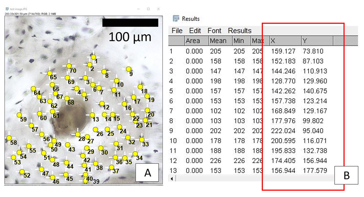
Figure 6
Screenshots of image analysis steps replicating our XY coordinate calculation protocol. A: secondary osteon with osteocyte lacunae (yellow dots). B: raw data output window in ImageJ/FIJI showing resulting XY coordinates (red rectangle).

Figure 7
Screenshot of final calculations of distances between XY coordinates yielded using the Medieval English histology sample. Column F, highlighted in yellow, shows the D values in μm. The line graph illustrates variation in D values from across the entire secondary osteon.
3. Disussion: interpretative value
We present here a simple and effective way to obtain an insight into the distances between neighbouring points in a 2D histology image (Figure 8). Those who regularly work with osteocyte lacunae or OPD data might already have raw data files from ImageJ/FIJI stored where the XY coordinates are saved. Certainly, whenever possible these should be provided alongside other commonly reported variables, either in the main body of an article or the online supplementary information. Re-analyses of data as outlined here may provide new insights into new or old research questions, although it is also vital to provide the sequence in which the points are counted. Very wide distances between some coordinates may simply reflect random and widespread counting across an image and thus have no meaning for understanding distances between neighbouring bone histology elements. To improve precision and minimise room for intra- and inter-observer error, we also suggest counts are placed at the most central point of each lacuna. Whilst doing this, it might be useful to make a note of lacuna morphology—whether the shapes are flat or round (van Oers, Wang & Bacabac 2015)—across all secondary osteons considered. This will help in future comparisons between different studies, and aid in the interpretation of distance data and osteocyte function within the broader context of research questions such as those relating to disease (van Oers, Wang & Bacabac 2015).
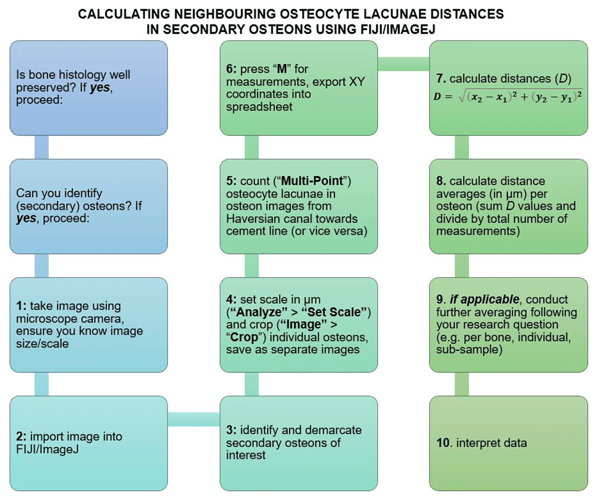
Figure 8
Flowchart summarising the steps of the protocol covered in our study. Please refer to text for more detail.
Researchers will need to pay close attention to the preservation of bone histology before considering examination at the osteocyte level. Our protocol will not yield meaningful results if any osteocyte lacunae are unidentifiable or obscured because of biodegradation or the effects of taphonomic agents. Generally, it is not easy to predict the histological level of preservation from the exterior of bone alone, or on the basis of its age in the archaeological or palaeontological context. For example, good osteocyte data have been gathered for dinosaurs (e.g., Stein & Werner 2013), but in more recent human and domesticated animal archaeological specimens they can be obliterated (e.g., Hollund et al. 2012; also see Jans 2008), which can seem counter-intuitive. We suggest testing ‘pilot’ samples before proceeding to create thin sections from larger assemblages.
The interpretative value of the distances between osteocyte lacunae on a path of counting is that it would inform how well inter-connected osteocytes were in a given sample, which can be applied to range of vertebrate specimens that show clear secondary osteons—direct products of bone remodelling—in their histology. This provides information about how actively bone was maintained (Andreaus, Colloca & Iacoviello 2014; Bromage et al. 2009), because the inter-connectedness of neighbouring lacunae facilitates healthy exchange of nutrients, bone biological signals, and fluid flow (Kollmannsberger et al. 2017; van Tol et al. 2020). To the best of our knowledge, there is no established range of osteocyte-to-osteocyte distance measurements for humans, or other animals, with most studies reporting experimental model data from independent projects. For example, Sugawara et al. (2005: 877) reported ~24 μm of “point-to-point distance between centers of the osteocytes” in embryonic chicks. Chen et al. (2018: 216) discussed 20–30 μm “osteocyte-to-osteocyte distance” as indicating effective dissemination of molecules throughout bone but they relied on Sugawara et al. (2005) for data. Jindrova, Tuma and Sladek (2016: 11) reported a range of ~17–33 μm “lacuna to lacuna distance” for Lurcher and wild type mice (average of ~27 μm in pooled mice), though the values depended on whether the measurements were from the periosteum, mid-cortex, or endosteum. Theoretical studies have used 30 μm of lacuna-to-lacuna distance in mathematical modelling of bone fluid flow, either citing anatomical literature that does not explicitly state where underlying data derive from (e.g., Goulet et al. (2009: 1392) rely on Chakkalakal (1989: 1038) where data are likely estimated based on canaliculi length); or mentioning preliminary “osteocyte-to-osteocyte” data from rat experiments without describing the methodology employed (Wang et al. 2000: 1202). In our Medieval human example, the resulting D values fell into the range reported in these studies. However, given the limited direct comparative data, interpretation of distances in future studies should focus on variation within- and between- specimens and creating baselines for a range of taxa. Nevertheless, bone micro-organisation is less influenced by phylogeny than it is by lifestyle, life history, and tissue/animal age (de Ricqlès 1993), so discussions based on animal experimental data are also reasonable.
Future research into osteocyte lacunae distance data could help further refine interpretations made from bone histology density and other geometric variables alone. For example, the study where femoral remodelling rates did not differ between Holocene and Pleistocene specimens (Streeter et al. 2010) was a follow up of an earlier study by Abbott, Trinkaus, and Burr (1996) using the same specimens. While Streeter et al. (2010) identified similarities in the density of secondary osteons, Abbott, Trinkaus, and Burr (1996) had noted differences in their geometric properties (the Pleistocene hominin samples had smaller osteon size than that measured in the Holocene specimens). This demonstrates variation can exist in how different histology variables quantify bone remodelling. Supplementing this with osteocyte lacunae distance data could clarify whether, despite the secondary osteon size differences, these hominins indeed maintained similar levels of remodelling but at the level of osteocytes. Further, including neighbouring osteocyte lacunae distance data in research that deals with species identification could assist in isolating humans from other mammals in forensic and archaeological commingled assemblages. Cummaudo et al. (2019) recently reported that osteocyte lacunae size changed with location within secondary osteons in the humerus, radius, ulna, femur, tibia, and fibula in one Medieval human and one pig (S. scrofa) sample. They also noted some statistically significant differences between human and pig samples in the size and circularity, but not in the number, of lacunae. However, they had sub-divided the secondary osteon regions into “inner, intermediate, and outer lacunae” (p. 713) instead of considering a continuous distribution of lacunae. Cummaudo et al. (2019) also included multiple bones per individual, which can be expanded to comparisons of osteocyte distribution depending on the long bone region (e.g., cortical vs trabecular bone, diaphysis vs metaphysis vs epiphysis) as was done by Canè et al. (1982). Cummaudo et al. (2019) only used one of each representative species, but their study shows potential for future exploration of osteocyte data for species identification, alongside other quantitative histology data.
The XY coordinate distance measurements may not be as useful in understanding secondary osteon distribution alone as they might be when applied to osteocyte lacunae, simply because osteons can remodel both stochastically and in a targeted fashion (Martin 2007), so it is almost impossible to determine the timing (sequence of secondary osteon appearance) of remodelling from post-mortem, archaeological, or fossilised bone samples. Identifying the timing of remodelling would also be difficult to achieve when dealing with bone from older individuals that show several generations of remodelled secondary osteons, possibly reflecting an OPD asymptote (Frost 1987). However, the technique could be applicable to counts of intact osteons (see Crowder et al. 2022) across a relatively larger image area (or a shaft cross-section) to determine whether BMU products were operating in a clustered or dispersed manner, alongside the osteon density data.
The key limitation of using the XY coordinate distance in bone histology examination is, of course, the 2D level of perspective which does not capture the 3D nature of osteocytes or osteonal structures in a bone sample (Andronowski & Cole 2021). Another limitation is that the outlined calculations need to be processed manually, in the sense that they have to be analysed outside of ImageJ/FIJI. However, once the main cell functions are set up, the XY coordinates from the ImageJ/FIJI output can be simply copied and pasted into a spreadsheet (a template is supplied in our Supplemental File). The advantage of using ImageJ/FIJI lies in having access to a forum of supporting scholars who are continually developing macros and plug-ins, and assist with coding, that can be used to calculate other XY coordinate distances that might be of interest to palaeohistologists (e.g., distance from centroid). Our protocol does not require significant training or access to expensive software and so would be applicable across a wide range of institutions, particularly where there is limited infrastructure (see Miszkiewicz 2020). While other disciplines can employ automated approaches to cell counting and measuring from larger 2D or 3D images (e.g., O’Driscoll et al. 1999), histologists working with archaeological or fossilised samples are hindered by issues with preservation, meaning that careful manual approaches to histology image analysis will continue to be needed. Being able to conduct manual XY coordinate counts could be a useful addition to the technical toolkit.
Additional File
The additional file for this article can be found as follows:
Supplementary file 1: Appendix
Raw data generated in this study. DOI: https://doi.org/10.5334/oq.117.s1
Acknowledgements
We thank the School of Social Science at the University of Queensland for access to microscopy facilities, and the University of Kent for facilitating access to the osteological collection in their care. We thank Matthew Law, Ariane Maggio, and Yasmine de Gruchy for helpful feedback which improved the original version of this article.
Funding Information
Australian Research Council (DE190100068); University of Kent (2010 Graduate Teaching Assistant PhD Scholarship).
Competing Interests
The authors have no competing interests to declare.
Author contributions
JJM designed study, conducted lab work, collected and analysed data, wrote first draft of the manuscript, secured funding; JL contributed to methodology and data analysis; PM: contributed materials, and to methodology. All edited manuscript.