
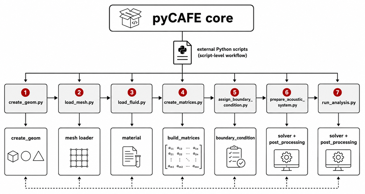
Figure 1
Overall architecture of the pyCAFE framework and main software modules.
Table 1
Eigenfrequency comparison between pyCAFE and the analytical solution for the rectangular rigid-wall cavity. Results are reported for CQUAD4 and CQUAD8 elements using the balanced mesh size .
| MODE (m, n) | fan [Hz] | fCQUAD4 [Hz] | [%] | fCQUAD8 [Hz] | [%] |
|---|---|---|---|---|---|
| (1,0) | 171.5000 | 171.8601 | 0.2099 | 171.5003 | 0.0002 |
| (0,1) | 343.0000 | 345.8854 | 0.8412 | 343.0096 | 0.0028 |
| (2,0) | 343.0000 | 345.8854 | 0.8412 | 343.0096 | 0.0028 |
| (1,1) | 383.4857 | 386.2287 | 0.7153 | 383.4944 | 0.0023 |
| (2,1) | 485.0753 | 489.1558 | 0.8412 | 485.0890 | 0.0028 |
| (3,0) | 514.5000 | 524.2622 | 1.8974 | 514.5717 | 0.0139 |
| (3,1) | 618.3520 | 628.0825 | 1.5736 | 618.4180 | 0.0107 |
| (0,2) | 686.0000 | 709.1965 | 3.3814 | 686.2968 | 0.0433 |
| (4,0) | 686.0000 | 709.1965 | 3.3814 | 686.2968 | 0.0433 |
| (1,2) | 707.1126 | 729.7229 | 3.1976 | 707.4009 | 0.0408 |
| Mean error | 1.6880% | 0.0163% | |||
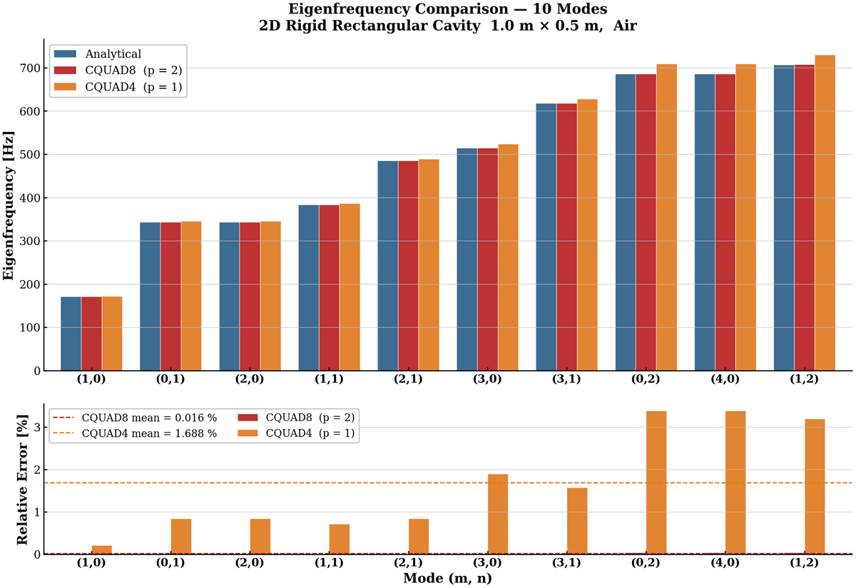
Figure 2
Histogram comparing the first 10 eigenfrequencies of the rectangular rigid-wall cavity obtained from the analytical solution, pyCAFE CQUAD4, and pyCAFE CQUAD8. The lower panel reports the relative error with respect to the analytical solution for the balanced mesh size .
Table 2
-refinement convergence study for the rectangular rigid-wall cavity. The table reports the number of nodes, the mean relative eigenfrequency error over the first 10 modes, and the corresponding solver time for CQUAD4 and CQUAD8 elements.
| h [m] | CQUAD4 | CQUAD8 | ||||
|---|---|---|---|---|---|---|
| NODES | MEAN ERR. [%] | TIME [s] | NODES | MEAN ERR. [%] | TIME [s] | |
| 0.200 | 18 | 10.2996 | 0.00 | 45 | 2.4886 | 0.01 |
| 0.140 | 40 | 5.8877 | 0.00 | 107 | 0.1851 | 0.01 |
| 0.100 | 66 | 3.3136 | 0.01 | 181 | 0.0606 | 0.02 |
| 0.070 | 120 | 1.6880 | 0.01 | 337 | 0.0163 | 0.04 |
| 0.050 | 231 | 0.8250 | 0.02 | 661 | 0.0040 | 0.09 |
| 0.035 | 450 | 0.4066 | 0.05 | 1305 | 0.0010 | 0.20 |
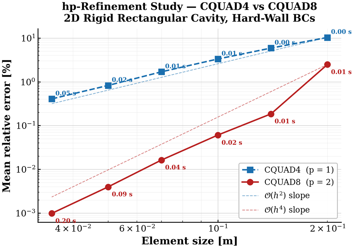
Figure 3
-refinement convergence of the mean eigenfrequency error over the first 10 modes. The dashed lines indicate the theoretical convergence rates for CQUAD4 and for CQUAD8. The solver time associated with each mesh is annotated next to the corresponding marker.
| pyCAFE | FEniCSx | |
|---|---|---|
| Element type | CQUAD8 serendipity () | Lagrange Q2 tensor-product |
| Mesh | Gmsh structured CQUAD8 | create_rectangle |
| DOFs, modal | 337 | 435 |
| Hard-wall BC | Natural Neumann | Natural Neumann |
Table 3
Comparison of the eigenfrequencies obtained with pyCAFE CQUAD8, FEniCSx Q2, and the analytical solution.
| MODE (m, n) | fan [Hz] | fFEniCSx [Hz] | [%] | fpyCAFE [Hz] | [%] |
|---|---|---|---|---|---|
| (1,0) | 171.5000 | 171.5003 | 0.0002 | 171.5003 | 0.0002 |
| (0,1) | 343.0000 | 343.0096 | 0.0028 | 343.0096 | 0.0028 |
| (2,0) | 343.0000 | 343.0096 | 0.0028 | 343.0096 | 0.0028 |
| (1,1) | 383.4857 | 383.4943 | 0.0023 | 383.4944 | 0.0023 |
| (2,1) | 485.0753 | 485.0888 | 0.0028 | 485.0890 | 0.0028 |
| (3,0) | 514.5000 | 514.5717 | 0.0139 | 514.5717 | 0.0139 |
| (3,1) | 618.3520 | 618.4170 | 0.0105 | 618.4180 | 0.0107 |
| (0,2) | 686.0000 | 686.2968 | 0.0433 | 686.2968 | 0.0433 |
| (4,0) | 686.0000 | 686.2968 | 0.0433 | 686.2968 | 0.0433 |
| (1,2) | 707.1126 | 707.4007 | 0.0407 | 707.4009 | 0.0408 |
| Mean error | 0.0163% | 0.0163% | |||
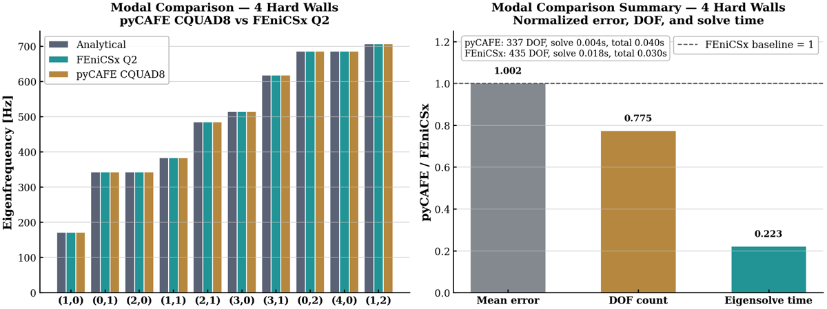
Figure 4
Left: Grouped bar chart of the first 10 eigenfrequencies obtained from the analytical solution, FEniCSx Q2, and pyCAFE CQUAD8. Right: Modal comparison summary normalised by the FEniCSx values. Ratios below one indicate smaller values for pyCAFE.
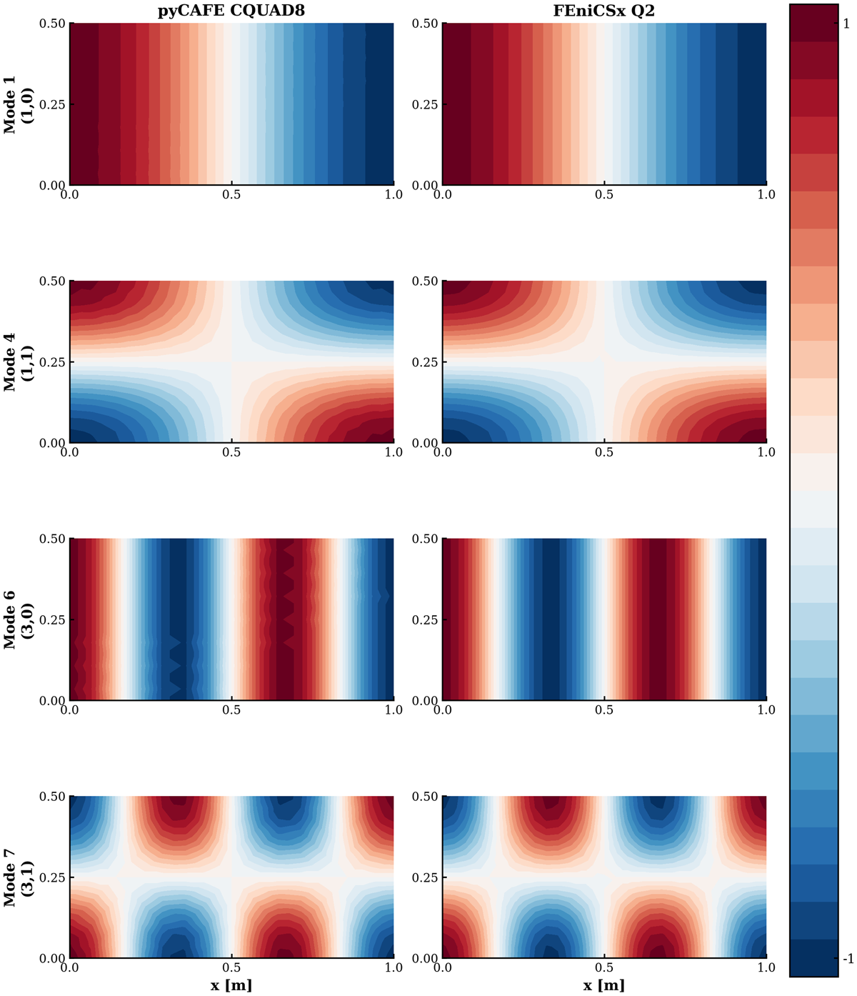
Figure 5
Mode-shape comparison between pyCAFE CQUAD8 and FEniCSx Q2 for modes 1, 4, 6 and 7.
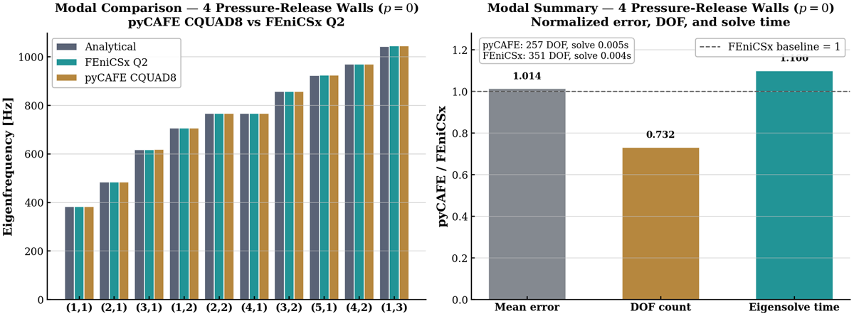
Figure 6
Left: Grouped bar chart of the first 10 eigenfrequencies for the zero pressure cavity, comparing the analytical solution, FEniCSx Q2, and pyCAFE CQUAD8. Right: Modal comparison metrics normalised by the FEniCSx values.
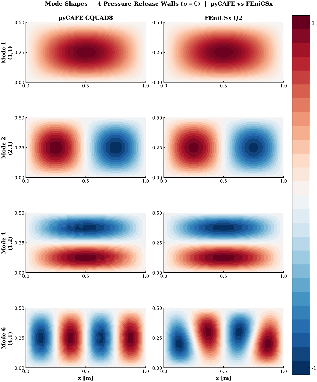
Figure 7
Mode-shape comparison between pyCAFE CQUAD8 and FEniCSx Q2 for modes 1, 2, 4 and 6 of the pressure-release cavity, with on all four walls. The comparison confirms that the two solvers reproduce the same spatial pressure patterns.
Table 4
Comparison of the eigenfrequencies obtained with pyCAFE CQUAD8, FEniCSx Q2, and the analytical solution for the pressure-release cavity with on all walls, using .
| MODE (m, n) | fan [Hz] | fFEniCSx [Hz] | [%] | fpyCAFE [Hz] | [%] |
|---|---|---|---|---|---|
| (1,1) | 383.4857 | 383.4943 | 0.0023 | 383.4944 | 0.0023 |
| (2,1) | 485.0753 | 485.0888 | 0.0028 | 485.0890 | 0.0028 |
| (3,1) | 618.3520 | 618.4170 | 0.0105 | 618.4180 | 0.0107 |
| (1,2) | 707.1126 | 707.4007 | 0.0407 | 707.4008 | 0.0408 |
| (2,2) | 766.9713 | 767.2411 | 0.0352 | 767.2438 | 0.0355 |
| (4,1) | 766.9713 | 767.2411 | 0.0352 | 767.2438 | 0.0355 |
| (3,2) | 857.5000 | 857.7805 | 0.0327 | 857.7932 | 0.0342 |
| (5,1) | 923.5558 | 924.3822 | 0.0895 | 924.3879 | 0.0901 |
| (4,2) | 970.1505 | 970.5703 | 0.0433 | 970.6082 | 0.0472 |
| (1,3) | 1043.1938 | 1045.3131 | 0.2032 | 1045.3136 | 0.2032 |
| Mean error | 0.0495% | 0.0502% | |||
Table 5
Eigenfrequencies, hard-wall cavity (Neumann walls), COMSOL versus pyCAFE CQUAD8 versus analytical ().
| MODE (m, n) | fan [Hz] | fCOMSOL [Hz] | [%] | fpyCAFE [Hz] | [%] |
|---|---|---|---|---|---|
| (1,0) | 171.5000 | 171.6020 | 0.0595 | 171.5003 | 0.0002 |
| (0,1) | 343.0000 | 343.2108 | 0.0615 | 343.0096 | 0.0028 |
| (2,0) | 343.0000 | 343.2131 | 0.0621 | 343.0096 | 0.0028 |
| (1,1) | 383.4857 | 383.7219 | 0.0616 | 383.4944 | 0.0023 |
| (2,1) | 485.0753 | 485.3750 | 0.0618 | 485.0890 | 0.0028 |
| (3,0) | 514.5000 | 514.8599 | 0.0699 | 514.5717 | 0.0139 |
| (3,1) | 618.3520 | 618.7697 | 0.0675 | 618.4180 | 0.0107 |
| (0,2) | 686.0000 | 686.6336 | 0.0924 | 686.2968 | 0.0433 |
| (4,0) | 686.0000 | 686.7041 | 0.1026 | 686.2968 | 0.0433 |
| (1,2) | 707.1126 | 707.8204 | 0.1001 | 707.4008 | 0.0408 |
| Mean error | 0.0739% | 0.0163% | |||
Table 6
Eigenfrequencies, zero pressure on all the four sides of the cavity ( on all walls), COMSOL versus pyCAFE CQUAD8 versus analytical ().
| MODE (m, n) | fan [Hz] | fCOMSOL [Hz] | [%] | fpyCAFE [Hz] | [%] |
|---|---|---|---|---|---|
| (1,1) | 383.4857 | 383.7219 | 0.0616 | 383.4944 | 0.0023 |
| (2,1) | 485.0753 | 485.3750 | 0.0618 | 485.0890 | 0.0028 |
| (3,1) | 618.3520 | 618.7697 | 0.0675 | 618.4180 | 0.0107 |
| (1,2) | 707.1126 | 707.8204 | 0.1001 | 707.4008 | 0.0408 |
| (2,2) | 766.9713 | 767.6333 | 0.0863 | 767.2438 | 0.0355 |
| (4,1) | 766.9713 | 767.6953 | 0.0944 | 767.2438 | 0.0355 |
| (3,2) | 857.5000 | 858.2792 | 0.0909 | 857.7932 | 0.0342 |
| (5,1) | 923.5558 | 924.7370 | 0.1279 | 924.3879 | 0.0901 |
| (4,2) | 970.1505 | 971.0964 | 0.0975 | 970.6082 | 0.0472 |
| (1,3) | 1043.1938 | 1045.9333 | 0.2626 | 1045.3136 | 0.2032 |
| Mean error | 0.1051% | 0.0502% | |||
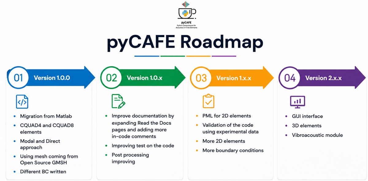
Figure 8
Roadmap of the future works for pyCAFE.