
(1) Overview
Introduction
Computational acoustics plays a central role in the numerical analysis of sound propagation in enclosed and semi-enclosed domains, such as ducts, cavities, and waveguides. In these applications, frequency domain formulations are widely adopted, particularly when time harmonic responses are of interest. For complex geometries and boundary conditions, analytical solutions are generally not available, making numerical approaches essential. Among the available numerical methods, the Finite Element Method (FEM) is commonly employed due to its ability to discretise arbitrary geometries and systematically incorporate a wide range of acoustic boundary conditions. The theoretical foundations of finite element formulations for acoustic problems are well established and extensively documented in the literature (1, 2, 3, 4, 5), building on general numerical concepts originally developed for structural mechanics and later extended to acoustics. Solving the acoustic field in enclosed and open domains is widely used in both academia and industry (6, 7, 8, 9). This work focuses on low- to mid-frequency analyses, namely the range in which the acoustic wavelength remains sufficiently large compared to the characteristic element size, and in which the coupling between the acoustic field and flexible structures is often most relevant. In this regime, structural resonances can interact strongly with the acoustic field, making the direct inspection of mass, stiffness, damping and boundary matrices particularly useful for validation and future vibroacoustic extensions (10, 11).
Although several open-source tools can solve Helmholtz-type problems, many of them rely on variational weak-form workflows, where the governing equations are expressed symbolically and assembled implicitly.
Among them, FEniCSx (12) currently represents one of the most widely used open-source environments for acoustic Helmholtz problems, also providing dedicated examples and modules for acoustic simulations within a general variational framework based on the Unified Form Language. FreeFEM (13) offers a scripting-based approach for finite element analysis on unstructured meshes, while scikit-fem (14) provides lightweight sparse matrix assembly in Python for general elliptic problems. However, the number of open-source tools specifically oriented toward educational and validation-focused acoustic FEM formulations remains limited. These frameworks differ from pyCAFE in scope and design philosophy. While general purpose Partial Differential Equations (PDE) environments are typically centred on high-level variational formulations, pyCAFE deliberately targets the two-dimensional acoustic Helmholtz equation through an element-based and matrix-based formulation. The global acoustic stiffness and mass matrices are assembled explicitly from element-level contributions, and the resulting operators are directly exposed to the user, together with explicit boundary condition matrices and a modal solver. It also mirrors the workflow of commercial FEM codes, making pyCAFE particularly suitable for educational and research-oriented use. The MATLAB predecessor CAFE (15) established this design philosophy; the present Python port extends accessibility while preserving numerical transparency. Subsequent developments showed that structural and acoustic domains may be assembled into a unified coupled system, enabling eigenvalue or time-harmonic analyses when required.
While coupled formulations and additional techniques, such as absorbing domains (16, 17, 18), represent important extensions of acoustic FEM, the present work focuses exclusively on two-dimensional acoustic problems. The authors recognise that several advanced features, including vibroacoustic coupling, absorbing boundary treatments, three-dimensional formulations, and additional element types and alternative solver strategies, can be incorporated in future versions. However, the purpose of this work is to establish a solid and well-validated foundation on which these developments can be built. For this reason, pyCAFE is deliberately introduced as a simple but transparent acoustic FEM framework, validated against analytical solutions, alternative numerical implementations and commercial finite element results.
The main contribution of pyCAFE is therefore not the introduction of a new finite element formulation, but the development of an open-source, matrix-based acoustic framework in Python. By exposing the assembled mass, stiffness, damping and boundary matrices, the software follows a philosophy that is close to common commercial FEM practice while remaining fully inspectable and modifiable by the user. This makes pyCAFE useful both for research, where transparent operators facilitate benchmarking and future extensions, and for education, where students and developers can directly examine the numerical structure of the Helmholtz problem.
The remainder of the paper is organised as follows. The Implementation and architecture section describes the structure of the software, the organisation of the core modules and the numerical workflow from mesh generation to post-processing. The Quality control section presents the testing strategy, the validation cases and the continuous integration workflow used to ensure reproducibility. The Availability section reports the repository, archive, operating system compatibility, programming language and software requirements. Finally, the Reuse Potential section discusses possible applications of pyCAFE, its current limitations and the planned extensions toward a broader open-source framework.
Implementation and architecture
The pyCAFE architecture is structured around a folder called core that oversees the simulation workflow and delegates particular duties to a group of modular subfolders. Figure 1 depicts a schematic overview of the software architecture.
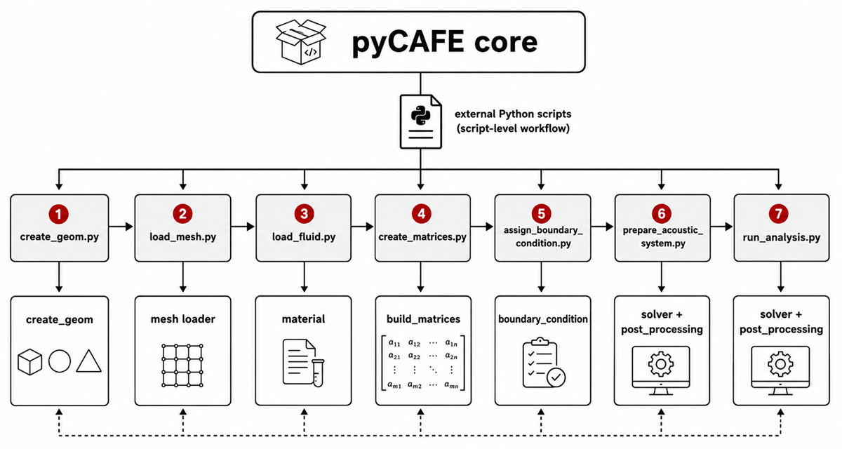
Figure 1
Overall architecture of the pyCAFE framework and main software modules.
The workflow is organised through Python scripts that import the required pyCAFE submodules, rather than embedding case-specific problem definitions within the core implementation. In this way, simulation parameters, boundary conditions and analysis options are specified at the script level, while the numerical routines remain separated from the user-defined configuration. This separation makes it possible to modify individual test cases without changing the underlying assembly and solution procedures. Geometry definition and mesh generation are performed outside the core solver. pyCAFE assumes that geometries are created according to a predefined syntax compatible with Gmsh input files (19). Auxiliary scripts are provided to support geometry creation, with particular attention to consistent naming conventions and physical group definitions. Once the mesh has been generated, it is imported through a dedicated loading module. The material properties of the acoustic medium are defined independently from the mesh, allowing the fluid parameters to be prescribed separately from the geometrical model. Boundary conditions are assigned through a different module, which currently supports interactive keyboard input. This choice keeps the boundary condition definition explicit and independent from the assembly routines. The resulting acoustic system is then passed to solver modules that support both direct frequency domain analyses and modal-based formulations. Post-processing utilities are used after the solution step to inspect and visualise acoustic pressure fields and derived quantities. Overall, the code structure separates geometry and mesh handling, material definition, boundary condition assignment, system assembly, solution and post-processing, so that each component can be inspected or modified independently.
Geometry and material selection
pyCAFE operates on externally generated two-dimensional meshes and includes auxiliary scripts that define the expected workflow for geometry creation, mesh generation and material parameter assignment. The geometry module currently supports the interactive definition of simple benchmark domains, namely rectangular and circular cavities, through keyboard input. The user specifies the geometrical parameters, the maximum frequency of interest and the desired element order, which can be either linear or quadratic.
Mesh generation is performed through the Gmsh Python API. In addition to defining the geometrical entities, the script assigns physical groups to the acoustic domain and to each boundary segment. To support reproducibility, the generated mesh is saved in a user-selected location through a file dialog. A companion mesh visualisation utility can then be used to load an existing .msh file, extract the node coordinates, element connectivities and physical boundary groups, and generate a two-dimensional plot for preliminary inspection.
The material properties of the acoustic medium are defined independently from the mesh. A dedicated material utility includes predefined parameter sets for common fluids, such as air and water, and also allows custom media to be defined by the user. The characteristic impedance,
is computed from the selected density and sound speed and returned together with these parameters, so that the same material definition is used consistently in the subsequent analysis steps.
Build matrices
The build matrices folder contains the numerical routines used to construct the acoustic finite element operators. This module implements the element formulations required to assemble the global stiffness, mass and damping matrices from the discretised mesh. Two quadrilateral acoustic elements are currently supported: the four-node element, referred to as CQUAD4, which uses a Gauss integration rule, and the eight-node quadratic element, referred to as CQUAD8, which uses a Gauss integration rule (20, 21).
Each element formulation is implemented in a dedicated module that contains the corresponding shape functions, Jacobian computation and element matrix construction. The element type is identified automatically from the imported mesh, and the appropriate formulation is then used during assembly. This avoids manual changes when switching between linear and quadratic discretisation. The separation between element formulations also keeps the implementation of each element self-contained and suitable for independent testing.
For regular acoustic fields in simple benchmark domains, CQUAD4 and CQUAD8 elements are expected to show convergence rates of and (22), respectively, according to standard finite element approximation theory (3, 4).
Boundary condition assignment
Boundaries are detected in the mesh, and the corresponding acoustic boundary condition is selected by the user. Multiple boundary condition types can therefore be assigned within the same model, according to the physical groups defined in the mesh. The assignment procedure is separated from both the solver and the matrix assembly routines, so that boundary conditions can be changed without modifying the numerical core.
The boundary condition module currently supports rigid, or so called hard wall boundaries, zero pressure boundaries, constant pressure boundaries, impedance boundaries and prescribed normal velocity boundaries. Rigid boundaries represent the default condition and impose zero normal particle velocity. Zero pressure and constant pressure boundaries prescribe the acoustic pressure along selected boundaries. Impedance boundaries relate pressure to normal particle velocity through a complex acoustic impedance, while prescribed normal velocity boundaries are used to represent vibrating surfaces or velocity-driven acoustic excitation. The treatment of boundary conditions distinguishes between two mathematically distinct types: natural or Neumann conditions and essential or Dirichlet conditions. Rigid walls, prescribed normal velocity and impedance boundaries are treated as natural boundary conditions, since they arise directly from the weak form of the Helmholtz equation. Rigid walls correspond to the homogeneous Neumann condition
In Eq. (2), is the acoustic pressure and is the outward normal direction to the boundary. This condition imposes zero normal pressure gradient and corresponds to zero normal particle velocity at a rigid wall.
A prescribed normal velocity contributes to the right-hand side vector through the boundary load term
In Eq. (3), is the load vector contribution associated with the prescribed normal velocity, i is the imaginary unit, is the angular frequency, is the density of the acoustic medium, is the prescribed normal particle velocity, is the boundary where the velocity condition is applied, is the vector of boundary shape functions and is the differential boundary length.
Impedance boundaries add an admittance weighted boundary contribution to the system matrix. The corresponding element contribution can be written as
and enters the dynamic stiffness matrix through the term
In Eqs.(4) and (5), is the impedance boundary matrix contribution associated with the local shape functions and , is the impedance boundary, and is the specific acoustic admittance. The specific acoustic admittance is defined as
In Eq.(6), is the normalised acoustic impedance, is the density of the acoustic medium and is the speed of sound.
Prescribed pressure boundaries are treated as essential boundary conditions and must be imposed explicitly on the algebraic system. In pyCAFE, zero pressure and non zero constant pressure boundaries are handled separately. Zero pressure boundaries are removed from the global system during assembly:
The rows and columns associated with these degrees of freedom are removed from , and , yielding the reduced operators
Non-zero pressure values are prescribed at selected degrees of freedom (DOF) and enforced through a partitioned formulation (23). The reduced system is split into known degrees of freedom, corresponding to the prescribed pressure values,
and unknown degrees of freedom. The resulting linear system is
In Eq.(10), is the vector of unknown pressure degrees of freedom, is the vector of prescribed pressure values, is the corresponding reduced load vector, is the block of the dynamic stiffness matrix associated with the unknown degrees of freedom, and couples the unknown degrees of freedom with the prescribed pressure degrees of freedom.
The reduced dynamic stiffness matrix is defined as
In Eq.(11), , and are the reduced stiffness, mass and damping matrices, respectively.
This treatment follows the standard static condensation procedure commonly used in matrix-based finite element formulations to impose prescribed degrees of freedom. Similar partitioning strategies are adopted in many finite element codes, where known degrees of freedom are separated from the unknowns before solving the reduced linear system.
In addition to boundary conditions defined along mesh boundaries, pyCAFE supports localised acoustic excitation through a point pressure source. The source is defined by its spatial coordinates, and the nearest mesh node is automatically identified. A pressure amplitude is then assigned to this node and included in the acoustic load vector. All boundary condition data are stored in a structured container, which is subsequently passed to the matrix assembly and solver routines.
Solver and post-processing
Once the global acoustic matrices and boundary contributions have been assembled, pyCAFE provides direct and modal solution strategies in the frequency domain. In the direct strategy, the acoustic response is computed independently at each frequency of interest. The final algebraic system is expressed through the dynamic stiffness matrix
where , and denote the assembled stiffness, mass and damping matrices after the application of the relevant boundary contributions. At each angular frequency , the complex pressure vector is obtained by solving
Sparse direct solvers are employed when available (24). This solution strategy is suitable when the full forced response is required over a prescribed frequency range.
In addition to the direct solution strategy, pyCAFE includes a modal solver for acoustic analysis. The solver computes natural frequencies and corresponding acoustic mode shapes by solving the generalised symmetric eigenvalue problem
The eigenproblem is solved using ARPACK through scipy.sparse.linalg.eigsh in shift invert mode. This formulation allows only the first eigenvalues and eigenvectors to be requested, which is appropriate for low- and mid-frequency studies where only a limited number of modes is required. The modal solver can be used for standalone modal studies or as a basis for reduced order models (25).
Post-processing utilities are provided to facilitate result interpretation. The acoustic pressure field can be reconstructed and visualised over the entire computational domain, while pressure values can also be extracted at specific spatial locations to obtain pointwise frequency response functions. Both amplitude and phase spectra are available and can be exported as plain text files containing the real part, imaginary part, modulus and phase of the complex pressure at the selected point.
An animated visualisation of the pressure field evolution across the analysed frequency range can also be generated as a video file. For modal analyses, individual acoustic mode shapes are reconstructed on the full mesh and displayed using a diverging colour map, which highlights nodal lines and pressure extrema. Finally, all field results, including frequency domain pressure distributions and acoustic mode shapes, can be exported in VTK Unstructured Grid (VTK = Visualization Toolkit) format together with a ParaView Data PVD collection file. This enables direct import into ParaView for interactive inspection and frequency by frequency visualisation.
Quality control
Automated test suite
The software is tested using pytest. The test suite includes approximately 70 tests organised into four categories, each implemented in a dedicated module:
Element matrices (test_element_matrices.py): Unit tests verifying symmetry of Ke and Me; the null-space condition (constant pressure is a free mode under Neumann boundary conditions); mass conservation (, where Ae is element area); partition of unity for shape functions (); and the Kronecker-delta interpolation property at element nodes. Tests are implemented for both CQUAD4 and CQUAD8 elements.
Boundary conditions (test_boundary_conditions.py): Tests verifying correct Dirichlet elimination via the partitioned system, correct identification of free-Degree of Freedom (DOF) index sets, and preservation of matrix symmetry after boundary condition application.
Modal solver (test_solver_modal.py): Validation of natural frequencies against the analytical closed- form solution for a rigid rectangular cavity, with mesh-dependent tolerances. Tests also verify monotone convergence of eigenvalues under mesh refinement and -orthogonality of the computed mode shapes.
Helmholtz solver (test_solver_helmholtz.py): Verification of the direct frequency domain solver on a reference problem with known pressure distribution.
Analytical validation and convergence
Rectangular rigid-wall cavity validation
The test domain is a two-dimensional rectangular acoustic cavity,
with dimensions and . The cavity is filled with air at . All four boundaries are modelled as rigid walls, corresponding to the homogeneous Neumann condition
This condition is naturally satisfied by the weak formulation and therefore does not require any modification of the assembled system matrices.
The discrete acoustic eigenvalue problem is written as
where and are the acoustic stiffness and mass matrices assembled element by element from the quadrilateral interpolation functions.
For a rigid rectangular cavity, the analytical eigenfrequencies are given by (26):
A mesh size of is used for the eigenfrequency comparison and for the histogram representation. This value lies in the middle of the convergence range, which will be discussed in the next section and provides a good compromise between numerical accuracy and computational cost. At this resolution, CQUAD8 already achieves a mean relative error below , whereas CQUAD4 requires a finer mesh to reach a comparable accuracy level.
Table 1 reports the first 10 eigenfrequencies computed by pyCAFE using CQUAD4 and CQUAD8 elements, and compares them with the analytical solution. The balanced mesh size is , corresponding to 120 nodes for CQUAD4 and 337 nodes for CQUAD8. The relative error is defined as
Figure 2 presents the same comparison in graphical form. The upper panel compares the absolute eigenfrequencies, while the lower panel reports the relative error with respect to the analytical solution.
Table 1
Eigenfrequency comparison between pyCAFE and the analytical solution for the rectangular rigid-wall cavity. Results are reported for CQUAD4 and CQUAD8 elements using the balanced mesh size .
| MODE (m, n) | fan [Hz] | fCQUAD4 [Hz] | [%] | fCQUAD8 [Hz] | [%] |
|---|---|---|---|---|---|
| (1,0) | 171.5000 | 171.8601 | 0.2099 | 171.5003 | 0.0002 |
| (0,1) | 343.0000 | 345.8854 | 0.8412 | 343.0096 | 0.0028 |
| (2,0) | 343.0000 | 345.8854 | 0.8412 | 343.0096 | 0.0028 |
| (1,1) | 383.4857 | 386.2287 | 0.7153 | 383.4944 | 0.0023 |
| (2,1) | 485.0753 | 489.1558 | 0.8412 | 485.0890 | 0.0028 |
| (3,0) | 514.5000 | 524.2622 | 1.8974 | 514.5717 | 0.0139 |
| (3,1) | 618.3520 | 628.0825 | 1.5736 | 618.4180 | 0.0107 |
| (0,2) | 686.0000 | 709.1965 | 3.3814 | 686.2968 | 0.0433 |
| (4,0) | 686.0000 | 709.1965 | 3.3814 | 686.2968 | 0.0433 |
| (1,2) | 707.1126 | 729.7229 | 3.1976 | 707.4009 | 0.0408 |
| Mean error | 1.6880% | 0.0163% | |||
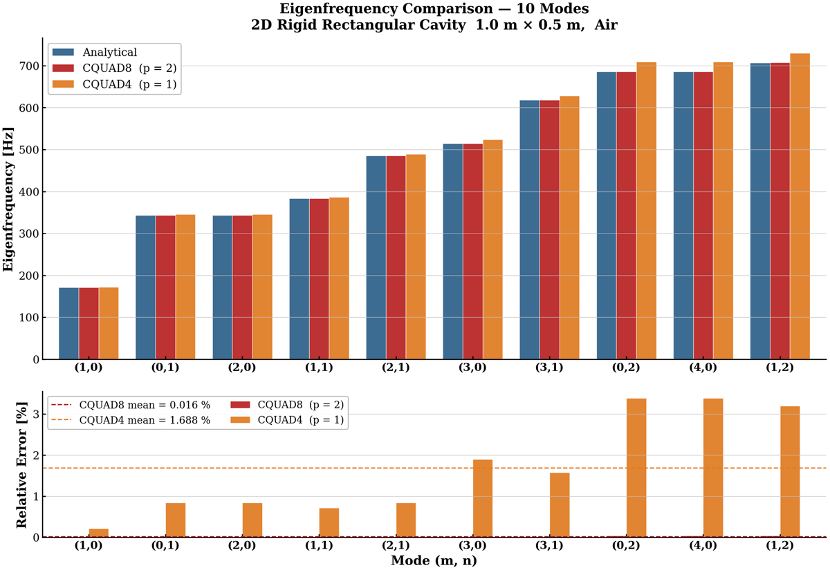
Figure 2
Histogram comparing the first 10 eigenfrequencies of the rectangular rigid-wall cavity obtained from the analytical solution, pyCAFE CQUAD4, and pyCAFE CQUAD8. The lower panel reports the relative error with respect to the analytical solution for the balanced mesh size .
hp-refinement convergence study
The convergence behaviour is assessed through an -refinement study. For a polynomial element of order , the eigenfrequency error is expected to scale as
Therefore, CQUAD4 elements, based on linear interpolation, are expected to show an convergence rate, while CQUAD8 elements, based on quadratic interpolation, are expected to show an convergence rate (27).
Table 2 reports the mean relative error over the first 10 modes for a sequence of mesh sizes. The balanced configuration, , is the mesh used for the eigenfrequency comparisons reported in the previous section. Figure 3 shows the corresponding convergence curves, together with the theoretical reference slopes and the solver time associated with each mesh.
Table 2
-refinement convergence study for the rectangular rigid-wall cavity. The table reports the number of nodes, the mean relative eigenfrequency error over the first 10 modes, and the corresponding solver time for CQUAD4 and CQUAD8 elements.
| h [m] | CQUAD4 | CQUAD8 | ||||
|---|---|---|---|---|---|---|
| NODES | MEAN ERR. [%] | TIME [s] | NODES | MEAN ERR. [%] | TIME [s] | |
| 0.200 | 18 | 10.2996 | 0.00 | 45 | 2.4886 | 0.01 |
| 0.140 | 40 | 5.8877 | 0.00 | 107 | 0.1851 | 0.01 |
| 0.100 | 66 | 3.3136 | 0.01 | 181 | 0.0606 | 0.02 |
| 0.070 | 120 | 1.6880 | 0.01 | 337 | 0.0163 | 0.04 |
| 0.050 | 231 | 0.8250 | 0.02 | 661 | 0.0040 | 0.09 |
| 0.035 | 450 | 0.4066 | 0.05 | 1305 | 0.0010 | 0.20 |
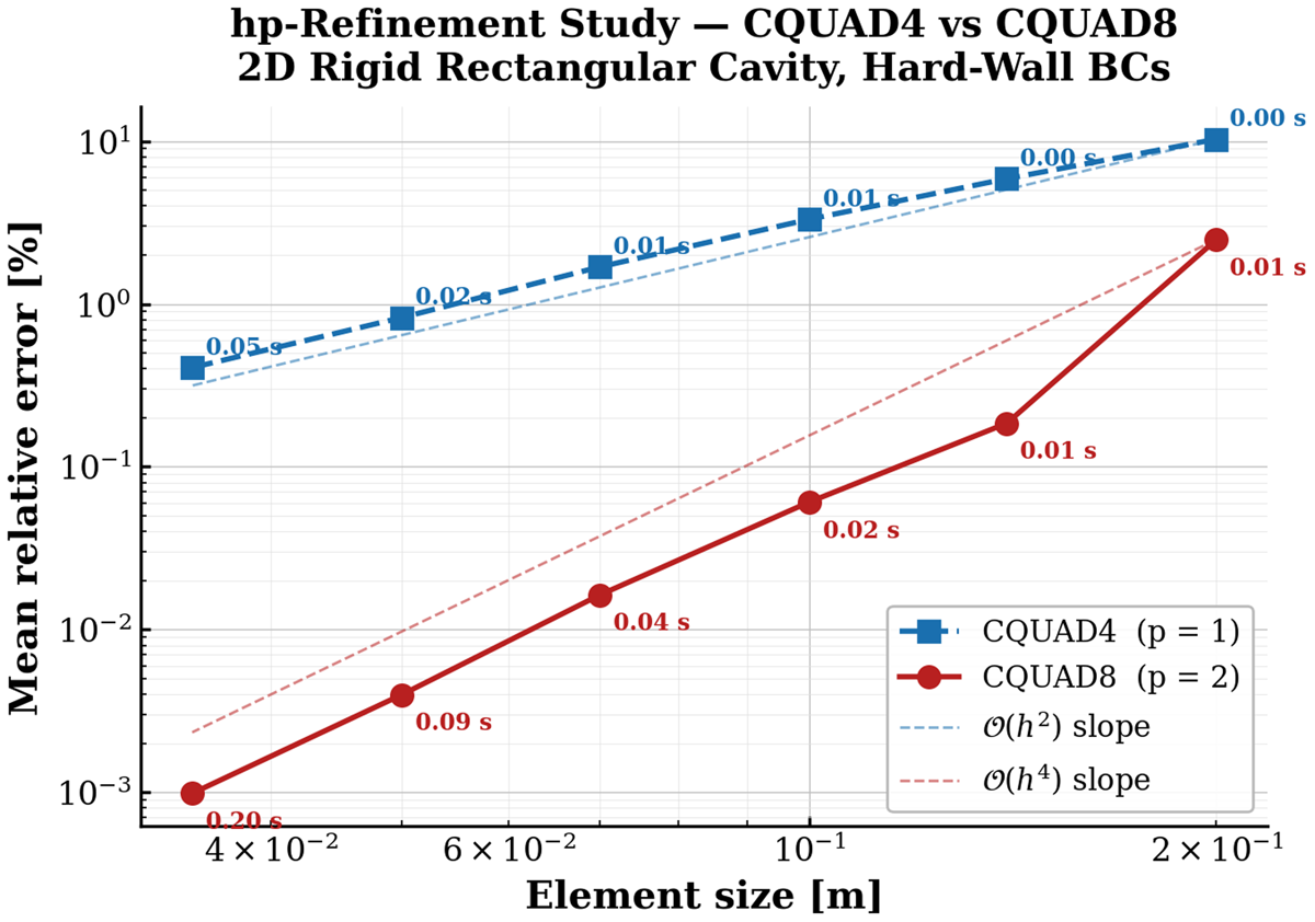
Figure 3
-refinement convergence of the mean eigenfrequency error over the first 10 modes. The dashed lines indicate the theoretical convergence rates for CQUAD4 and for CQUAD8. The solver time associated with each mesh is annotated next to the corresponding marker.
Comparison with FEniCSx
The pyCAFE results are cross-validated against FEniCSx(DOLFINx v0.9), an established open-source FEM platform, using the same cavity geometry and a balanced mesh configuration. The objective of this section is twofold: first, to verify that pyCAFE reproduces the same physical solution, and second, to quantify whether this agreement is obtained at a comparable or lower computational cost.
| pyCAFE | FEniCSx | |
|---|---|---|
| Element type | CQUAD8 serendipity () | Lagrange Q2 tensor-product |
| Mesh | Gmsh structured CQUAD8 | create_rectangle |
| DOFs, modal | 337 | 435 |
| Hard-wall BC | Natural Neumann | Natural Neumann |
Modal analysis with hard walls
Table 3 compares the first 10 eigenfrequencies. For the balanced configuration, pyCAFE and FEniCSx achieve the same mean relative error to four significant digits, namely 0.0163%, in both cases. However, pyCAFE reaches this accuracy with 337 pressure unknowns instead of 435 for FEniCSx, corresponding to approximately 22.5% fewer DOFs. In addition, the reduced eigensolve stage is faster in pyCAFE, with a computational time of 0.004 s compared with 0.018 s for FEniCSx. This corresponds to a speed ratio of 4.48 in favour of pyCAFE for this test case. Figure 4 summarises the corresponding normalised error, DOF count, and eigensolve time metrics.
Table 3
Comparison of the eigenfrequencies obtained with pyCAFE CQUAD8, FEniCSx Q2, and the analytical solution.
| MODE (m, n) | fan [Hz] | fFEniCSx [Hz] | [%] | fpyCAFE [Hz] | [%] |
|---|---|---|---|---|---|
| (1,0) | 171.5000 | 171.5003 | 0.0002 | 171.5003 | 0.0002 |
| (0,1) | 343.0000 | 343.0096 | 0.0028 | 343.0096 | 0.0028 |
| (2,0) | 343.0000 | 343.0096 | 0.0028 | 343.0096 | 0.0028 |
| (1,1) | 383.4857 | 383.4943 | 0.0023 | 383.4944 | 0.0023 |
| (2,1) | 485.0753 | 485.0888 | 0.0028 | 485.0890 | 0.0028 |
| (3,0) | 514.5000 | 514.5717 | 0.0139 | 514.5717 | 0.0139 |
| (3,1) | 618.3520 | 618.4170 | 0.0105 | 618.4180 | 0.0107 |
| (0,2) | 686.0000 | 686.2968 | 0.0433 | 686.2968 | 0.0433 |
| (4,0) | 686.0000 | 686.2968 | 0.0433 | 686.2968 | 0.0433 |
| (1,2) | 707.1126 | 707.4007 | 0.0407 | 707.4009 | 0.0408 |
| Mean error | 0.0163% | 0.0163% | |||
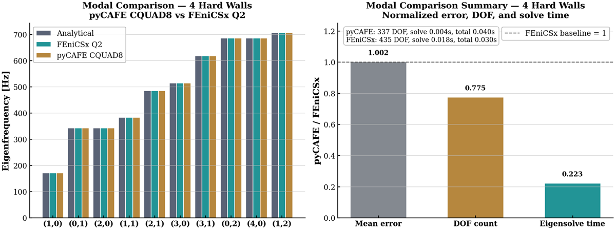
Figure 4
Left: Grouped bar chart of the first 10 eigenfrequencies obtained from the analytical solution, FEniCSx Q2, and pyCAFE CQUAD8. Right: Modal comparison summary normalised by the FEniCSx values. Ratios below one indicate smaller values for pyCAFE.
To complement the eigenfrequency comparison, Figure 5 compares the corresponding pressure mode shapes for modes 1, 4, 6 and 7 computed with the two solvers. Each field is normalised to the interval , so that the visual comparison focuses on the nodal pattern and phase distribution rather than on the absolute scaling.
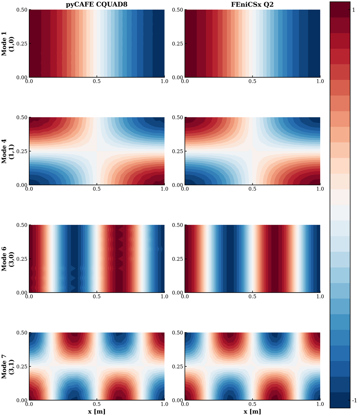
Figure 5
Mode-shape comparison between pyCAFE CQUAD8 and FEniCSx Q2 for modes 1, 4, 6 and 7.
Modal analysis with zero pressure walls
As a second modal benchmark, all four walls are assigned a homogeneous Dirichlet condition, , turning the domain into a pressure-release cavity. In pyCAFE, this boundary condition is handled by the built-in Guyan reduction (23), where the boundary nodes are eliminated from the system before the eigensolve. In FEniCSx, the same reduction is applied by extracting the free degrees of freedom before calling the sparse eigenvalue solver.
Table 4 reports the first 10 eigenfrequencies. Both solvers achieve very low errors, with a mean error of 0.0502% for pyCAFE and 0.0495% for FEniCSx. pyCAFE requires 257 reduced DOFs, while FEniCSx requires 351 free DOFs. In this pressure-release configuration, the reduced eigensolve stage is slightly slower in pyCAFE than in FEniCSx. However, the accuracy remains essentially the same for the two solvers, confirming that the Dirichlet reduction adopted in pyCAFE preserves the expected modal behaviour. Figure 6 reports the corresponding summary chart, following the same format used for the rigid-wall case. To further assess the spatial structure of the numerical solution, Figure 7 also compares selected pressure mode shapes obtained with the two solvers.
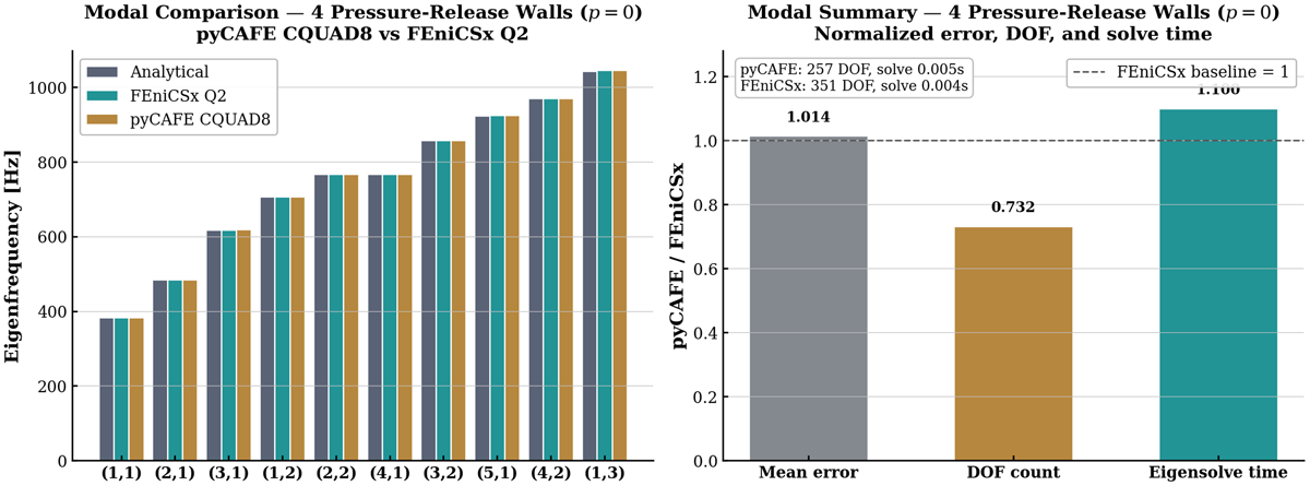
Figure 6
Left: Grouped bar chart of the first 10 eigenfrequencies for the zero pressure cavity, comparing the analytical solution, FEniCSx Q2, and pyCAFE CQUAD8. Right: Modal comparison metrics normalised by the FEniCSx values.
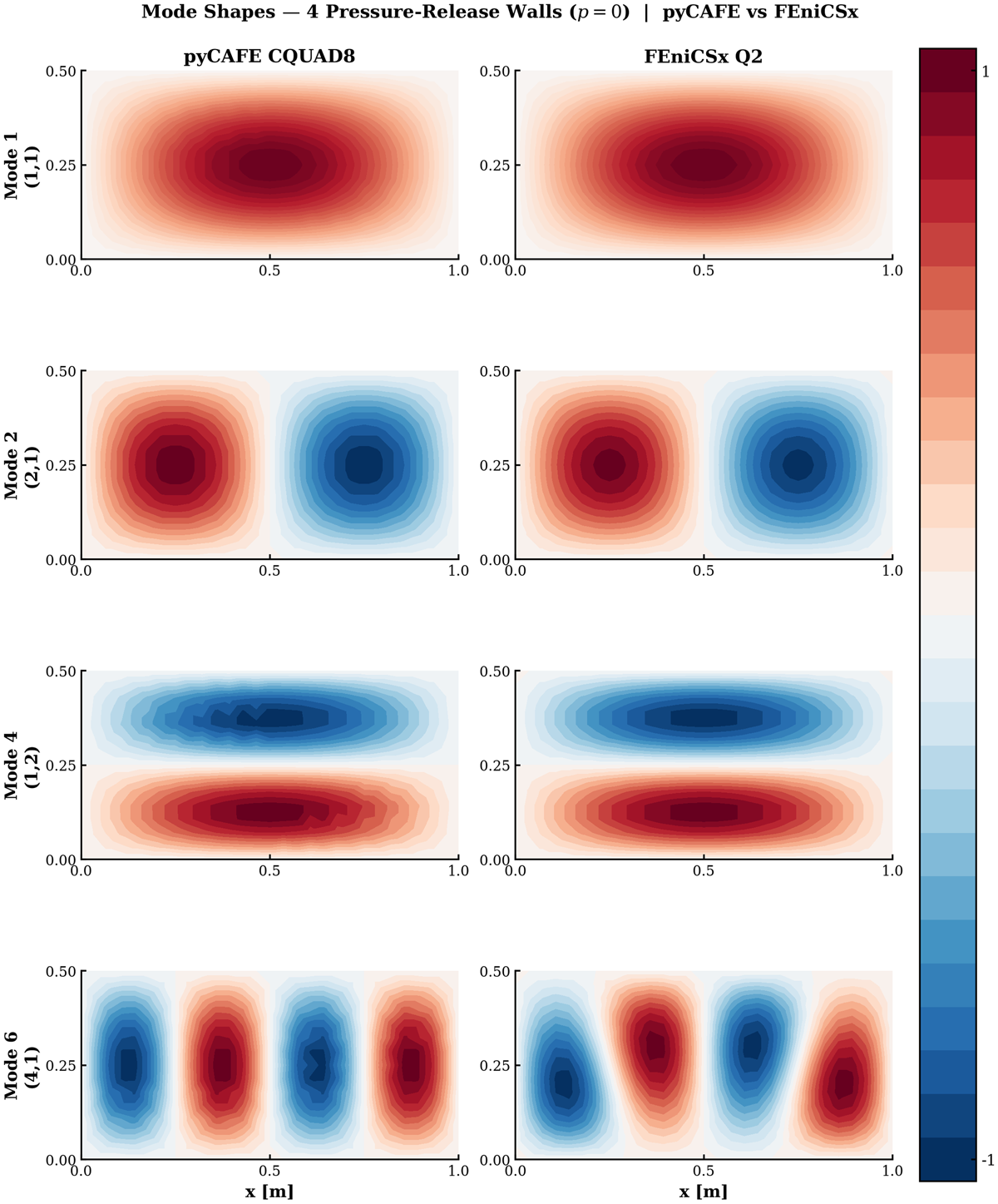
Figure 7
Mode-shape comparison between pyCAFE CQUAD8 and FEniCSx Q2 for modes 1, 2, 4 and 6 of the pressure-release cavity, with on all four walls. The comparison confirms that the two solvers reproduce the same spatial pressure patterns.
Table 4
Comparison of the eigenfrequencies obtained with pyCAFE CQUAD8, FEniCSx Q2, and the analytical solution for the pressure-release cavity with on all walls, using .
| MODE (m, n) | fan [Hz] | fFEniCSx [Hz] | [%] | fpyCAFE [Hz] | [%] |
|---|---|---|---|---|---|
| (1,1) | 383.4857 | 383.4943 | 0.0023 | 383.4944 | 0.0023 |
| (2,1) | 485.0753 | 485.0888 | 0.0028 | 485.0890 | 0.0028 |
| (3,1) | 618.3520 | 618.4170 | 0.0105 | 618.4180 | 0.0107 |
| (1,2) | 707.1126 | 707.4007 | 0.0407 | 707.4008 | 0.0408 |
| (2,2) | 766.9713 | 767.2411 | 0.0352 | 767.2438 | 0.0355 |
| (4,1) | 766.9713 | 767.2411 | 0.0352 | 767.2438 | 0.0355 |
| (3,2) | 857.5000 | 857.7805 | 0.0327 | 857.7932 | 0.0342 |
| (5,1) | 923.5558 | 924.3822 | 0.0895 | 924.3879 | 0.0901 |
| (4,2) | 970.1505 | 970.5703 | 0.0433 | 970.6082 | 0.0472 |
| (1,3) | 1043.1938 | 1045.3131 | 0.2032 | 1045.3136 | 0.2032 |
| Mean error | 0.0495% | 0.0502% | |||
To further support reproducibility, additional direct-frequency-response comparisons between pyCAFE and FEniCSx are provided in the examples and validation folders of the GitHub repository. These examples are intended for users interested in inspecting the direct Helmholtz sweep cases and the corresponding boundary condition implementations.
Comparison with commercial software
To implement the pyCAFE validation, the same cavity is also compared against COMSOL Multiphysics 6.2. Two modal datasets are considered: rigid walls, corresponding to a hard-wall Neumann condition, and zero pressure walls on all four sides. As reported in Tables 5 and 6, pyCAFE provides slightly lower frequency errors than COMSOL for both boundary condition configurations. This result confirms that the matrix-based implementation adopted in pyCAFE can reproduce the analytical modal solution with accuracy at least comparable to, and in this benchmark slightly higher than, that obtained with a commercial finite element package.
Table 5
Eigenfrequencies, hard-wall cavity (Neumann walls), COMSOL versus pyCAFE CQUAD8 versus analytical ().
| MODE (m, n) | fan [Hz] | fCOMSOL [Hz] | [%] | fpyCAFE [Hz] | [%] |
|---|---|---|---|---|---|
| (1,0) | 171.5000 | 171.6020 | 0.0595 | 171.5003 | 0.0002 |
| (0,1) | 343.0000 | 343.2108 | 0.0615 | 343.0096 | 0.0028 |
| (2,0) | 343.0000 | 343.2131 | 0.0621 | 343.0096 | 0.0028 |
| (1,1) | 383.4857 | 383.7219 | 0.0616 | 383.4944 | 0.0023 |
| (2,1) | 485.0753 | 485.3750 | 0.0618 | 485.0890 | 0.0028 |
| (3,0) | 514.5000 | 514.8599 | 0.0699 | 514.5717 | 0.0139 |
| (3,1) | 618.3520 | 618.7697 | 0.0675 | 618.4180 | 0.0107 |
| (0,2) | 686.0000 | 686.6336 | 0.0924 | 686.2968 | 0.0433 |
| (4,0) | 686.0000 | 686.7041 | 0.1026 | 686.2968 | 0.0433 |
| (1,2) | 707.1126 | 707.8204 | 0.1001 | 707.4008 | 0.0408 |
| Mean error | 0.0739% | 0.0163% | |||
Table 6
Eigenfrequencies, zero pressure on all the four sides of the cavity ( on all walls), COMSOL versus pyCAFE CQUAD8 versus analytical ().
| MODE (m, n) | fan [Hz] | fCOMSOL [Hz] | [%] | fpyCAFE [Hz] | [%] |
|---|---|---|---|---|---|
| (1,1) | 383.4857 | 383.7219 | 0.0616 | 383.4944 | 0.0023 |
| (2,1) | 485.0753 | 485.3750 | 0.0618 | 485.0890 | 0.0028 |
| (3,1) | 618.3520 | 618.7697 | 0.0675 | 618.4180 | 0.0107 |
| (1,2) | 707.1126 | 707.8204 | 0.1001 | 707.4008 | 0.0408 |
| (2,2) | 766.9713 | 767.6333 | 0.0863 | 767.2438 | 0.0355 |
| (4,1) | 766.9713 | 767.6953 | 0.0944 | 767.2438 | 0.0355 |
| (3,2) | 857.5000 | 858.2792 | 0.0909 | 857.7932 | 0.0342 |
| (5,1) | 923.5558 | 924.7370 | 0.1279 | 924.3879 | 0.0901 |
| (4,2) | 970.1505 | 971.0964 | 0.0975 | 970.6082 | 0.0472 |
| (1,3) | 1043.1938 | 1045.9333 | 0.2626 | 1045.3136 | 0.2032 |
| Mean error | 0.1051% | 0.0502% | |||
(2) Availability
Operating system
This package is compatible with macOS, Windows, and Linux operating systems supporting Python version 3.10 or newer. No operating system-specific features are required. Compatibility across Python 3.10, 3.11, and 3.12 is verified automatically via the GitHub Actions CI pipeline on every commit.
Programming language
The software is implemented in Python (version ). All core functionalities, including mesh handling, matrix assembly, solvers, and post-processing utilities, are written in Python.
Additional system requirements
No special hardware requirements are imposed. The software can be executed on standard desktop or laptop computers. Memory and CPU requirements scale with the size of the finite element model; typical two-dimensional acoustic problems with a few thousand degrees of freedom can be solved on consumer-grade hardware.
Dependencies
The following Python packages are required for basic functionality:
NumPy ( 1.20) (28): Numerical arrays and vectorised operations
SciPy ( 1.8) (29): Sparse linear algebra routines and frequency domain solvers
Matplotlib ( 3.5) (30): Visualisation and post-processing of acoustic fields
tqdm ( 4.60): Progress monitoring for frequency sweeps
Gmsh ( 4.10) (19): Geometry definition and finite element mesh generation via the Python API
The package can be installed directly from PyPI: pip install pycafe
List of contributors
Daniele Fabbri: Conceptualisation, software development, numerical implementation, validation and manuscript preparation.
Fabio Bruzzone: Scientific supervision, methodological guidance and critical review of the numerical approach and software design.
Carlo Rosso: Scientific supervision, methodological guidance and critical review of the numerical approach and software design.
Software location
Code repository (GitHub)
Name: pyCAFE
Persistent identifier: https://github.com/DanFabb/pycafe
Licence: MIT License
Date published: 19/12/2025
Archived software version (Zenodo)
Name: pyCAFE
Persistent identifier: https://doi.org/10.5281/zenodo.19599893
Date published: 15/04/2026
Language
English
(3) Reuse Potential
The pyCAFE framework is designed for acoustic analyses in two-dimensional domains discretised with finite elements. Its main target to simulate typical applications include enclosed cavities, ducts and generic two-dimensional acoustic domains generated from external meshes. The software supports both direct frequency domain analyses and modal approaches, making it suitable for resonance studies, frequency sweeps, validation exercises and lightweight research simulations.
The reuse potential of pyCAFE is mainly associated with three contexts: education, numerical benchmarking and research prototyping. Its modular structure allows new finite elements, boundary conditions and solution strategies to be added by extending the relevant submodules without altering the general workflow.
Educational use
Two example notebooks are provided to guide users through the main analysis workflows. The notebook examples/Example_Modal.ipynb presents an eigenvalue analysis of a rectangular acoustic cavity. It builds a structured quadrilateral mesh using Gmsh, imports the mesh into pyCAFE, allows the user to assign boundary conditions wall by wall through an interactive interface, assembles the reduced acoustic system, and solves for the first prescribed number of natural frequencies and mode shapes. The results can be inspected through two-dimensional Matplotlib plots of the normalised pressure modes, inline PyVista visualisation, or optional export to VTK for post-processing in ParaView. This example is therefore intended to answer the question of what the resonant frequencies of the cavity are and what the associated acoustic pressure modes look like.
The notebook examples/Example_Direct_Sweep.ipynb presents the corresponding forced response workflow. It uses the same mesh generation and boundary condition interface, but solves the Helmholtz problem over a prescribed frequency range instead of solving an eigenvalue problem. The user can visualise the pressure field at selected frequencies, inspect the solution in PyVista, extract a probe response as a frequency response function, save the response to frf_probe.txt, and optionally export the full pressure fields to Visualization Toolkit (VTK). This example is therefore intended to show how the acoustic pressure field and point response vary under harmonic excitation.
Benchmarking and cross-validation
The matrix-based formulation makes pyCAFE a lightweight reference implementation for benchmarking acoustic finite element procedures. Since the stiffness, mass and boundary contribution matrices are explicitly assembled, they can be extracted and compared with independent codes at operator level.
Two validation paths are documented:
Analytical validation: Eigenfrequencies of a rigid rectangular cavity are compared with the closed-form solution, as reported in Table 1. Relative errors below are obtained with CQUAD8 elements.
FEniCSx Q2 validation: Modal eigenfrequencies are compared with an independent FEniCSx implementation. The corresponding mode shapes, shown in Figures 5 and 7, demonstrate the close agreement between the two formulations for both all Neumann and pressure-release configurations. In addition, the repository includes a dedicated validation notebook that performs a direct Helmholtz frequency response comparison between pyCAFE and FEniCSx. This provides an additional verification path for the forced response solver, although the corresponding results are not reported in the present paper.
These tests cover both eigenvalue and direct solution procedures, as well as all Neumann and mixed boundary condition configurations. The same validation structure can be reused to test additional element formulations, boundary conditions, or solver options by adding the corresponding module and running the existing test suite.
Research simulation
For research applications, pyCAFE provides a self-contained Python workflow for parametric acoustic studies in the frequency domain. The direct solver supports single frequency analyses and broadband sweeps with impedance, velocity, or pressure boundary conditions. The modal solver provides natural frequencies and mode shapes, which can also be used as a reduced order basis for efficient parametric analyses (25).
The two example notebooks illustrate these complementary workflows. Example_Modal.ipynb focuses on free acoustic response, resonance frequencies and mode shapes, while Example_Direct_Sweep.ipynb focuses on forced harmonic response, pressure field reconstruction and frequency response functions. Together, they provide reusable templates for setting up new cavity or duct simulations starting from a Gmsh mesh and a user-defined set of boundary conditions.
Future work
Planned developments beyond version 1.0.1 are summarised in Figure 8. They include:
Three-dimensional elements: Extension to hexahedral elements, such as HEX8 and HEX20, and tetrahedral elements for three-dimensional acoustic cavities and enclosures.
Perfectly matched layers: Implementation of absorbing regions for unbounded domain and radiation problems in two dimensions (31).
Time domain solver: Addition of explicit and implicit time integration schemes for transient acoustic problems.
Vibroacoustic coupling: Implementation of structural acoustic coupling through the assembly of a combined fluid structure system within the existing matrix-based framework (10).
Extended post-processing: Computation of sound power, directivity maps, and export to standard data formats.
Conda distribution: The package is currently available on PyPI through pip install pycafe, while a Conda package is planned.
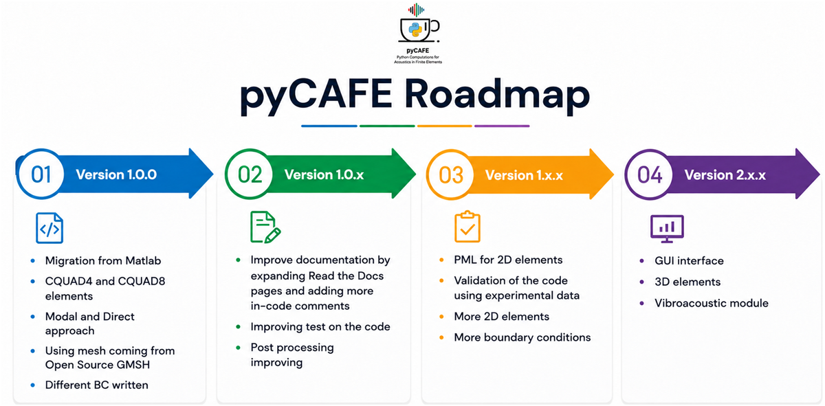
Figure 8
Roadmap of the future works for pyCAFE.
Contributions from the community are encouraged. Users interested in extending the software are invited to open an issue or submit a pull request through the public code repository.
Author Contributions
Daniele Fabbri - Conceptualisation, software development, numerical implementation, validation, and manuscript preparation.
Fabio Bruzzone - Supervision and critical review of the manuscript.
Carlo Rosso - Supervision and critical review of the manuscript.