
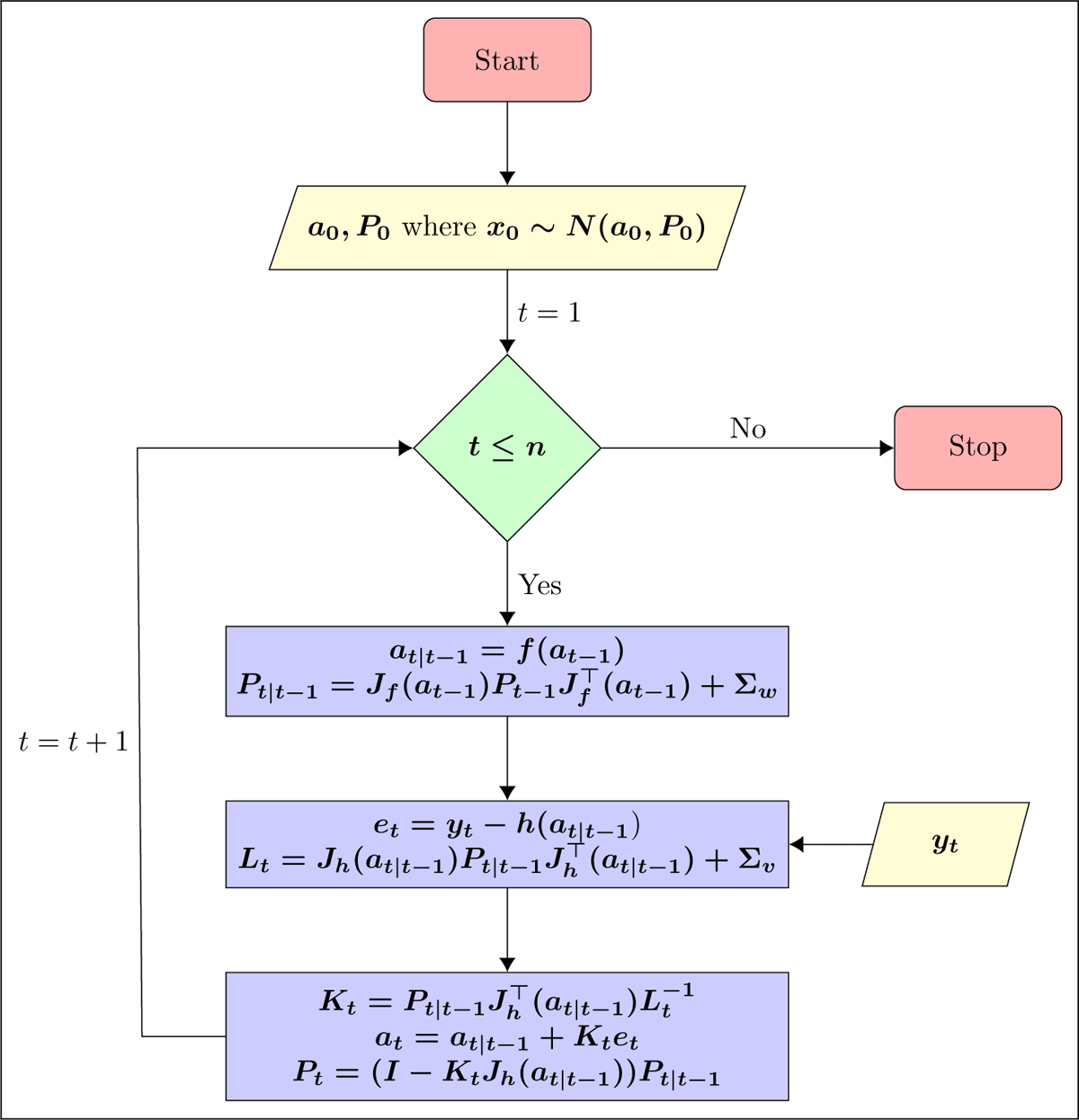
Figure 1
Flowchart of EKF.
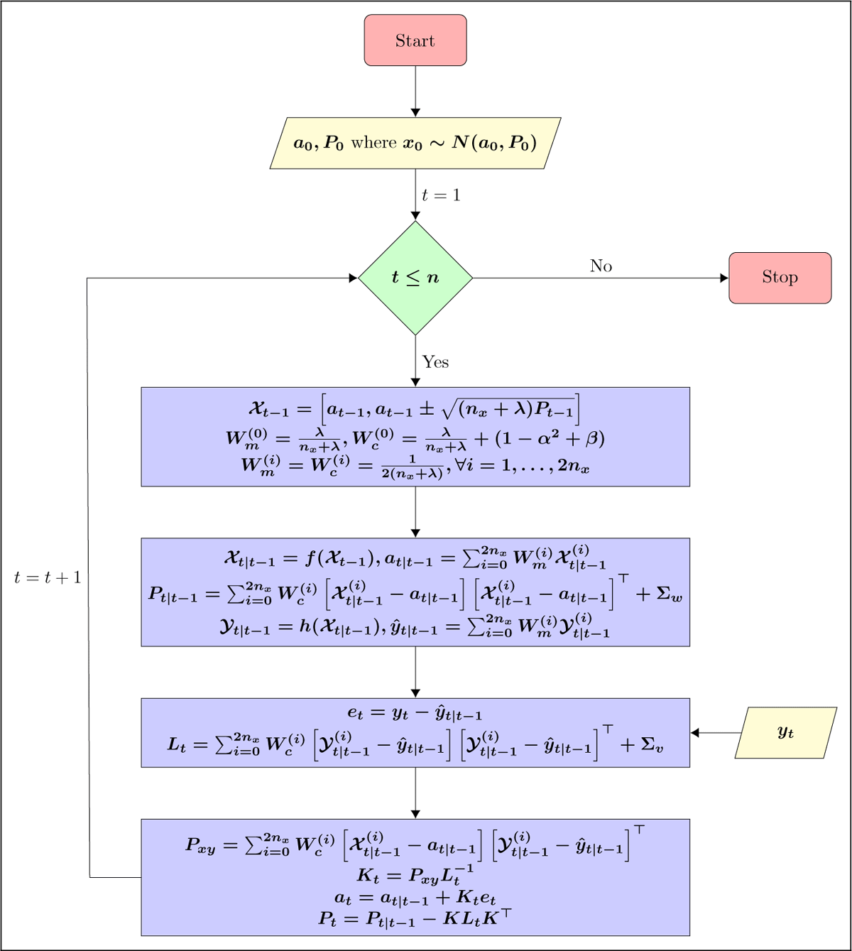
Figure 2
Flowchart of UKF.

Figure 3
Establish global configurations.

Figure 4
Specify model parameters (Schwartz-Smith model).

Figure 5
Download simulated data.
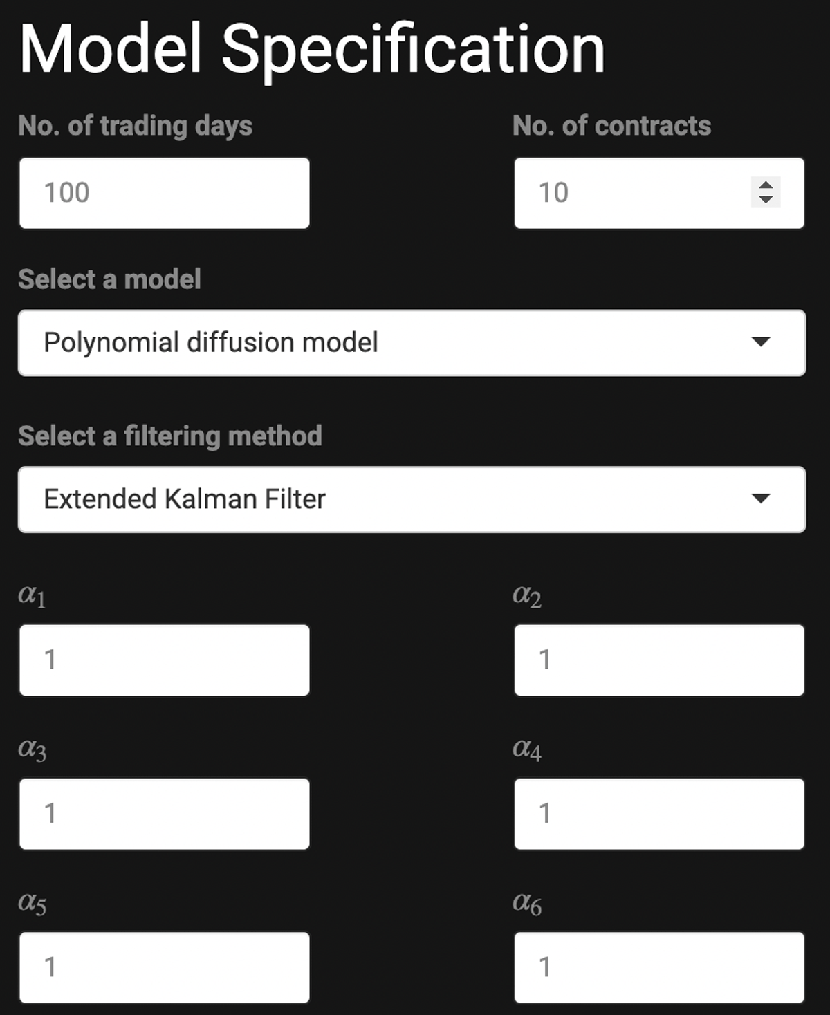
Figure 6
Specify model parameters (polynomial diffusion model).
Table 1
Estimation mean absolute errors of the logarithm of futures prices with different maturities.
| Maturity | SS paper | PDSim – SS MODEL | PDSim – PD MODEL |
|---|---|---|---|
| 1 month | 0.0314 | 0.0268 | 0.0519 |
| 5 months | 0.0035 | 0.0005 | 0.0279 |
| 9 months | 0.0020 | 0.0030 | 0.0290 |
| 13 months | 0.0000 | 0.0000 | 0.0338 |
| 17 months | 0.0028 | 0.0038 | 0.0410 |
Table 2
Root mean square errors (RMSE) for each futures contract using the polynomial diffusion (PD) model and the Schwartz-Smith (SS) model for the period from 2015 to 2018.
| CONTRACTS | PDSim – PD MODEL | PDSim – SS MODEL |
|---|---|---|
| Contract 1 | 1.1481 | 0.8884 |
| Contract 2 | 0.7283 | 0.5043 |
| Contract 3 | 0.4262 | 0.2460 |
| Contract 4 | 0.2522 | 0.1189 |
| Contract 5 | 0.1347 | 0.0614 |
| Contract 6 | 0.0516 | 0.0903 |
| Contract 7 | 0.0136 | 0.1056 |
| Contract 8 | 0.0323 | 0.1080 |
| Contract 9 | 0.0385 | 0.0963 |
| Contract 10 | 0.0251 | 0.0708 |
| Contract 11 | 0.0018 | 0.0526 |
| Contract 12 | 0.0322 | 0.0611 |
| Contract 13 | 0.0693 | 0.0933 |
| Mean | 0.2272 | 0.1921 |