
Table 1
Toy dataset for comparison of two groups. Dependent variable is working memory capacity.
| 65-YEAR OLDS | day 1 | day 2 | 75-year olds | day 1 | day 2 |
|---|---|---|---|---|---|
| Participant 1 | 42 | 40 | Participant 11 | 27 | 27 |
| Participant 2 | 23 | 23 | Participant 12 | 35 | 37 |
| Participant 3 | 44 | 46 | Participant 13 | 43 | 43 |
| Participant 4 | 20 | 20 | Participant 14 | 51 | 49 |
| Participant 5 | 43 | 47 | Participant 15 | 19 | 25 |
| Participant 6 | 37 | 37 | Participant 16 | 52 | 50 |
| Participant 7 | 48 | 46 | Participant 17 | 34 | 34 |
| Participant 8 | 53 | 53 | Participant 18 | 24 | 26 |
| Participant 9 | 50 | 52 | Participant 19 | 35 | 35 |
| Participant 10 | 33 | 33 | Participant 20 | 23 | 21 |
Table 2
Data of the toy dataset after averaging the scores of day 1 and day 2.
| 65-YEAR OLDS | SCORE | 75-year olds | SCORE |
|---|---|---|---|
| Participant 1 | 41 | Participant 11 | 27 |
| Participant 2 | 23 | Participant 12 | 36 |
| Participant 3 | 45 | Participant 13 | 43 |
| Participant 4 | 20 | Participant 14 | 50 |
| Participant 5 | 45 | Participant 15 | 22 |
| Participant 6 | 37 | Participant 16 | 51 |
| Participant 7 | 47 | Participant 17 | 34 |
| Participant 8 | 53 | Participant 18 | 25 |
| Participant 9 | 51 | Participant 19 | 35 |
| Participant 10 | 33 | Participant 20 | 22 |
| M = 39.5 | M = 34.5 | ||
| SD = 11.23 | SD = 10.78 |
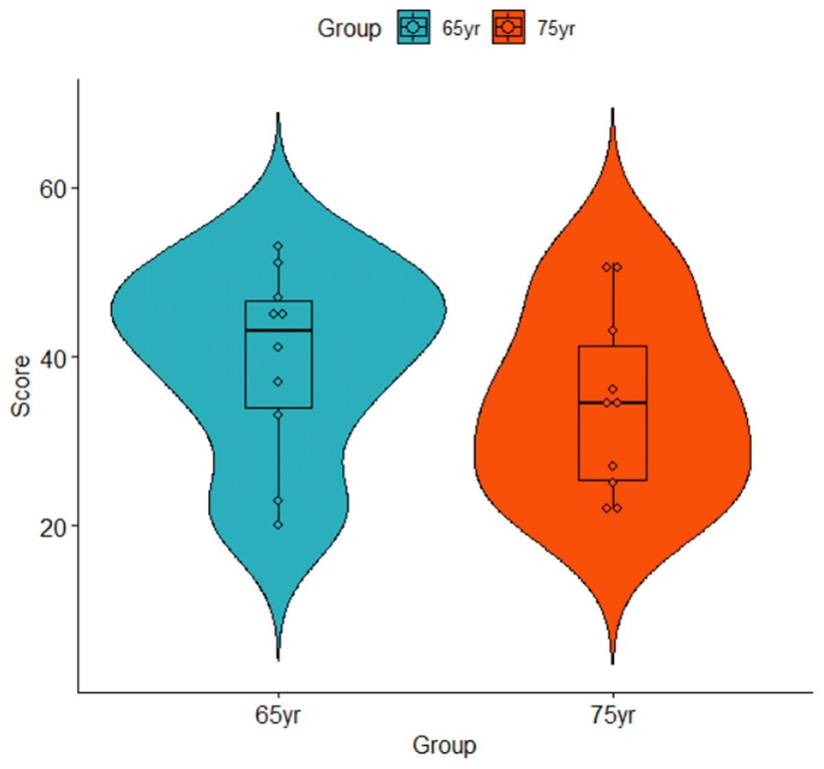
Figure 1
Violin plot of the data listed in Table 2.
Table 3
Long format input to run the t-test in R and in jamovi. Make sure you have 20 lines (2 groups * 10 participants in each group).
| PARTICIPANT | GROUP | SCORE |
|---|---|---|
| Participant 1 | 65yr | 41 |
| Participant 2 | 65yr | 23 |
| Participant 3 | 65yr | 45 |
| Participant 4 | 65yr | 20 |
| Participant 5 | 65yr | 45 |
| Participant 6 | 65yr | 37 |
| Participant 7 | 65yr | 47 |
| Participant 8 | 65yr | 53 |
| Participant 9 | 65yr | 51 |
| Participant 10 | 65yr | 33 |
| Participant 11 | 75yr | 27 |
| Participant 12 | 75yr | 36 |
| Participant 13 | 75yr | 43 |
| Participant 14 | 75yr | 50 |
| Participant 15 | 75yr | 22 |
| Participant 16 | 75yr | 51 |
| Participant 17 | 75yr | 34 |
| Participant 18 | 75yr | 25 |
| Participant 19 | 75yr | 35 |
| Participant 20 | 75yr | 22 |
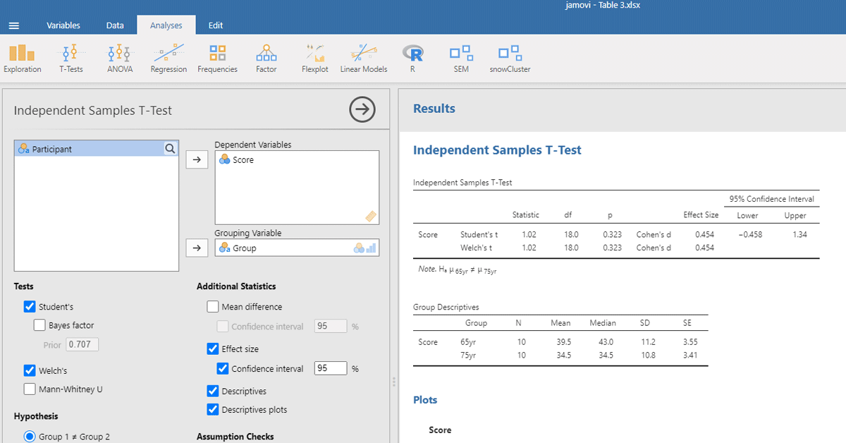
Figure 2
jamovi output for the t-test of working memory capacity between two age groups.
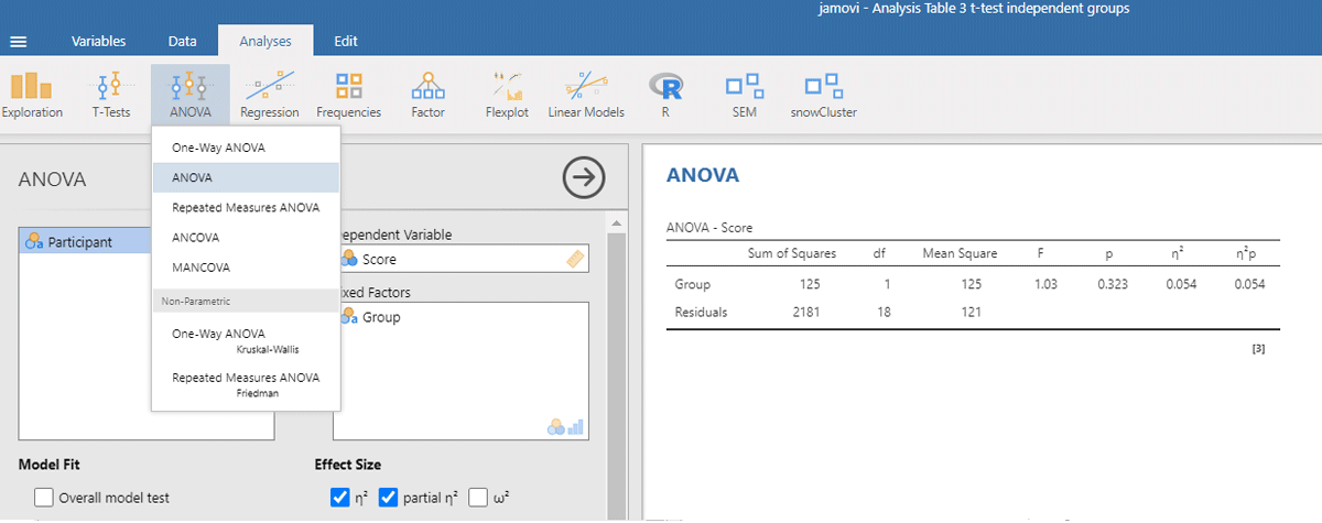
Figure 3
Output jamovi ANOVA between-groups analysis working memory capacity.
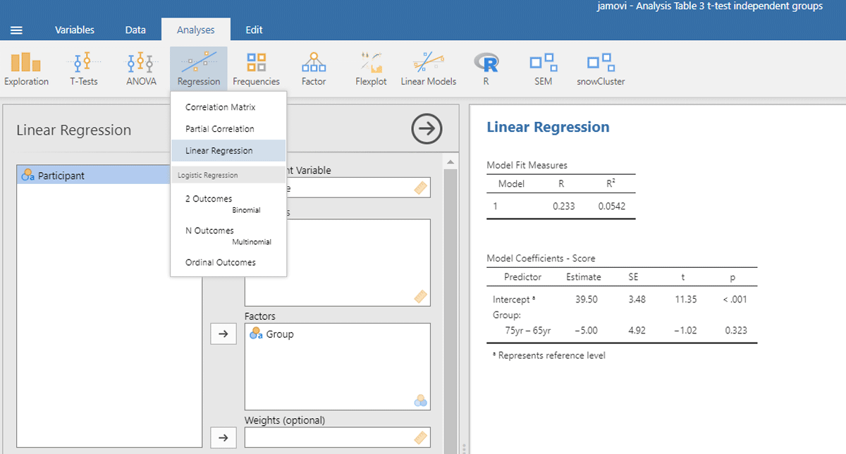
Figure 4
Output jamovi linear regression analysis of between-groups example working memory.
Table 4
Outline of the input file for an LME analysis in R and jamovi (total number of data lines is 40: 20 participants * 2 days).
| PARTICIPANT | GROUP | TIME | SCORE |
|---|---|---|---|
| Participant 1 | 65yr | day1 | 42 |
| Participant 1 | 65yr | day2 | 40 |
| Participant 2 | 65yr | day1 | 23 |
| Participant 2 | 65yr | day2 | 23 |
| … |
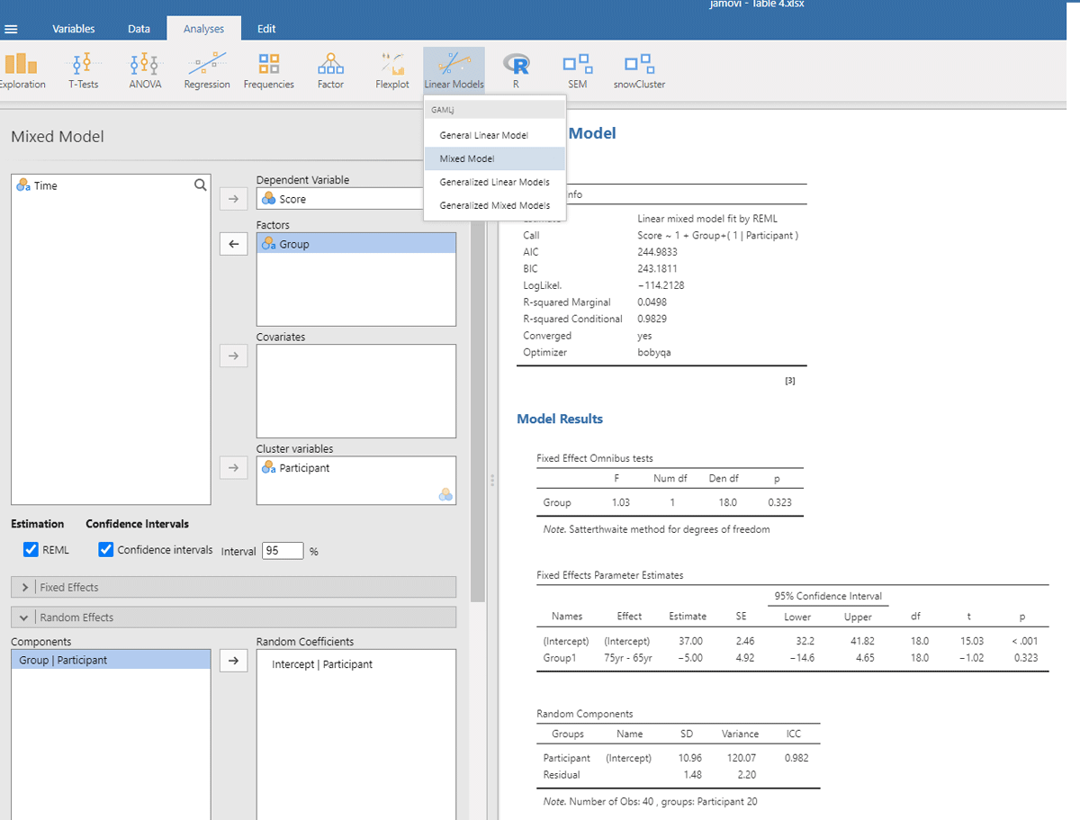
Figure 5
Output jamovi LME analysis of between-groups example working memory.
Table 5
Longitudinal data of a group of participants tested twice (day 1 & 2) at different ages (65 & 75 years). Dependent variable is working memory capacity.
| PARTICIPANT | 65yr day 1 | 65yr day 2 | 75yr day 1 | 75yr day 2 |
|---|---|---|---|---|
| Participant 1 | 32 | 30 | 27 | 27 |
| Participant 2 | 38 | 42 | 35 | 37 |
| Participant 3 | 42 | 38 | 43 | 43 |
| Participant 4 | 57 | 55 | 51 | 49 |
| Participant 5 | 24 | 30 | 19 | 25 |
| Participant 6 | 57 | 49 | 52 | 50 |
| Participant 7 | 37 | 39 | 34 | 34 |
| Participant 8 | 33 | 33 | 24 | 26 |
| Participant 9 | 40 | 38 | 35 | 35 |
| Participant 10 | 22 | 20 | 23 | 21 |
Table 6
Table for a t-test repeated measure example working memory.
| PARTICIPANT | 65yr | 75yr | diff |
|---|---|---|---|
| Participant 1 | 31 | 27 | 4 |
| Participant 2 | 40 | 36 | 4 |
| Participant 3 | 40 | 43 | –3 |
| Participant 4 | 56 | 50 | 6 |
| Participant 5 | 27 | 22 | 5 |
| Participant 6 | 53 | 51 | 2 |
| Participant 7 | 38 | 34 | 4 |
| Participant 8 | 33 | 25 | 8 |
| Participant 9 | 39 | 35 | 4 |
| Participant 10 | 21 | 22 | –1 |
| M65 = 37.8 | M75 = 34.5 | Mdiff = 3.3 | |
| SD65 = 10.76 | SD75 = 10.78 | SDdiff = 3.23 |
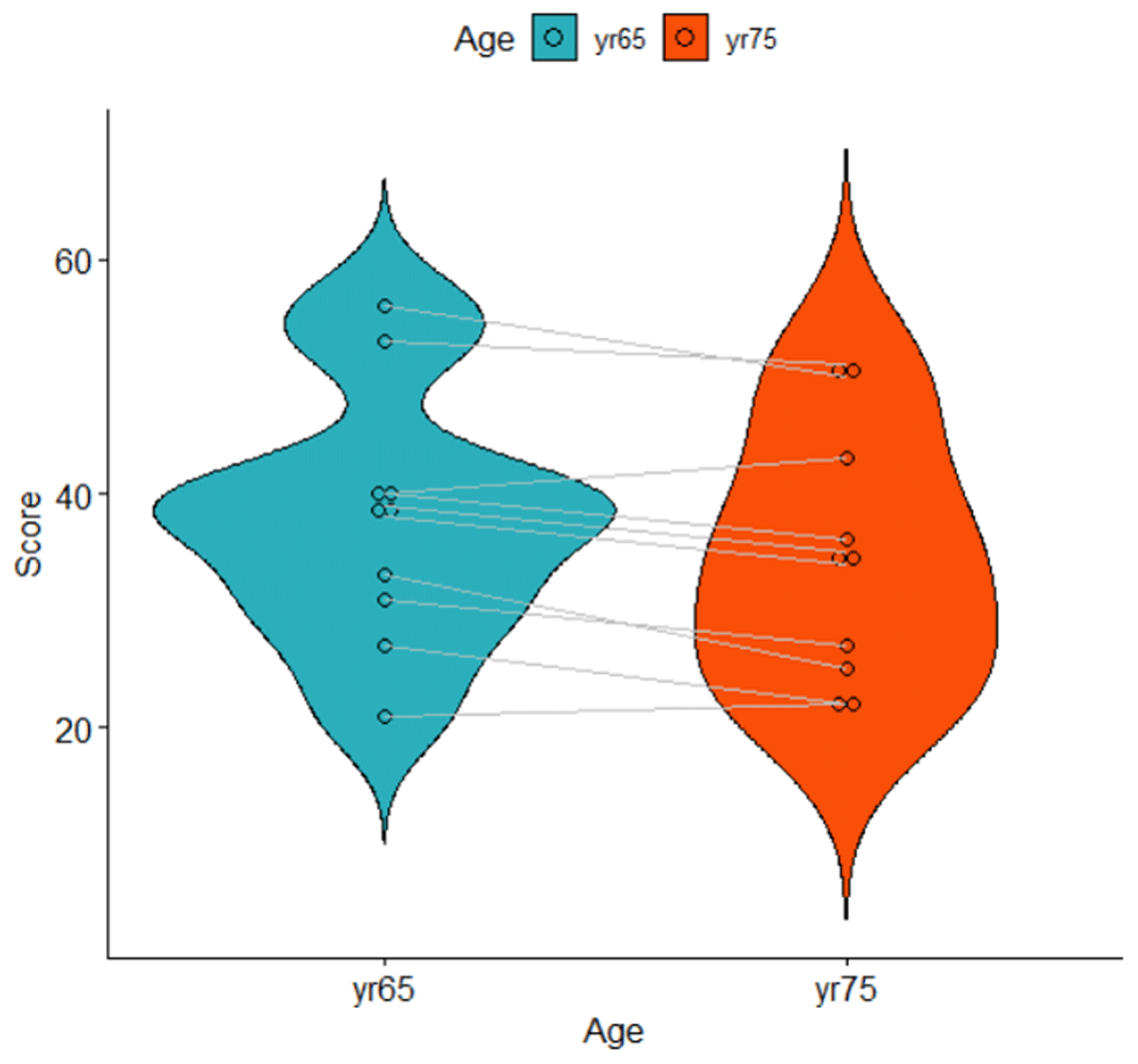
Figure 6
Violin plot of the data shown in Table 6. Lines represent related observations.
Table 7
Input for R and jamovi analysis of t-test related samples.
| PARTICIPANT | yr65 | yr75 |
|---|---|---|
| Participant 1 | 31 | 27 |
| Participant 2 | 40 | 36 |
| Participant 3 | 40 | 43 |
| Participant 4 | 56 | 50 |
| Participant 5 | 27 | 22 |
| Participant 6 | 53 | 51 |
| Participant 7 | 38 | 34 |
| Participant 8 | 33 | 25 |
| Participant 9 | 39 | 35 |
| Participant 10 | 21 | 22 |
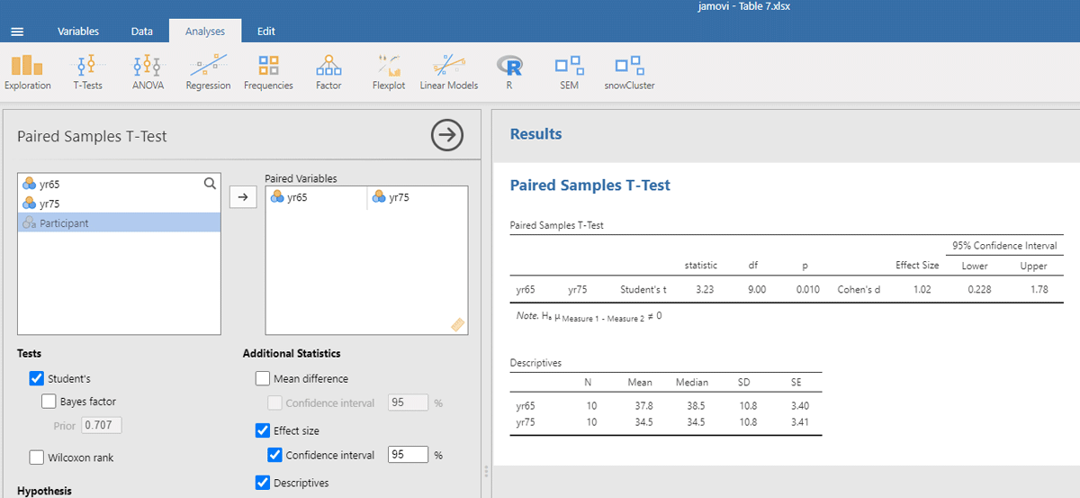
Figure 7
Output jamovi t-test longitudinal study working memory.
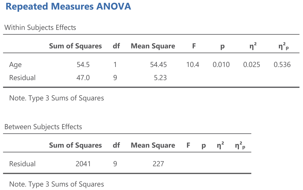
Figure 8
Output jamovi ANOVA longitudinal study working memory.
Table 8
Long format version of Table 5, needed as input for LME analysis related samples (must contain a total of 40 data rows: 10 participants * 2 ages * 2 days tested).
| PARTICIPANT | AGE | DAY | SCORE |
|---|---|---|---|
| Participant 1 | yr65 | day1 | 32 |
| Participant 2 | yr65 | day1 | 38 |
| Participant 3 | yr65 | day1 | 42 |
| Participant 4 | yr65 | day1 | 57 |
| Participant 5 | yr65 | day1 | 24 |
| Participant 6 | yr65 | day1 | 57 |
| Participant 7 | yr65 | day1 | 37 |
| Participant 8 | yr65 | day1 | 33 |
| Participant 9 | yr65 | day1 | 40 |
| Participant 10 | yr65 | day1 | 22 |
| Participant 1 | yr65 | day2 | 30 |
| … | |||
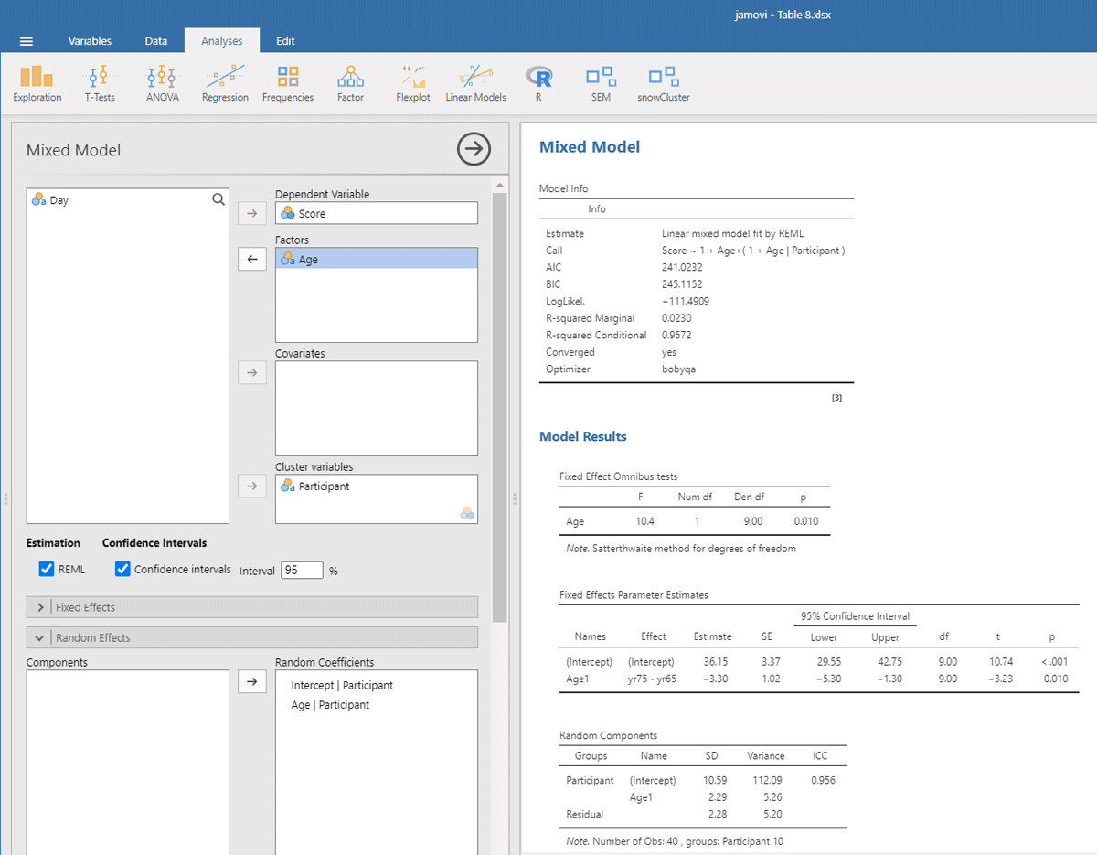
Figure 9
Output jamovi LME analysis longitudinal study working memory.
Table 9
Data of an experiment with two repeated measure variables (Day and Stimulus type) and two measurements per condition. Dependent variable is a hypothetical variable.
| PARTICIPANT | DAY 1 | DAY 2 | ||||||
|---|---|---|---|---|---|---|---|---|
| STIMULUS TYPE 1 | STIMULUS TYPE 2 | STIMULUS TYPE 1 | STIMULUS TYPE 2 | |||||
| MEAS1 | MEAS2 | MEAS1 | MEAS2 | MEAS1 | MEAS2 | MEAS1 | MEAS2 | |
| Participant 1 | 3 | 3 | 5 | 5 | 5 | 3 | 1 | 4 |
| Participant 2 | 5 | 7 | 4 | 7 | 4 | 5 | 4 | 3 |
| Participant 3 | 4 | 3 | 4 | 4 | 5 | 6 | 2 | 3 |
| Participant 4 | 1 | 2 | 4 | 5 | 6 | 5 | 3 | 2 |
| Participant 5 | 6 | 4 | 8 | 8 | 8 | 9 | 7 | 9 |
| Participant 6 | 5 | 4 | 5 | 7 | 7 | 7 | 5 | 6 |
| Participant 7 | 6 | 6 | 7 | 7 | 7 | 4 | 8 | 5 |
| Participant 8 | 4 | 4 | 5 | 3 | 6 | 4 | 5 | 4 |
| Participant 9 | 5 | 3 | 6 | 3 | 5 | 6 | 6 | 7 |
| Participant 10 | 7 | 8 | 9 | 7 | 7 | 9 | 8 | 9 |
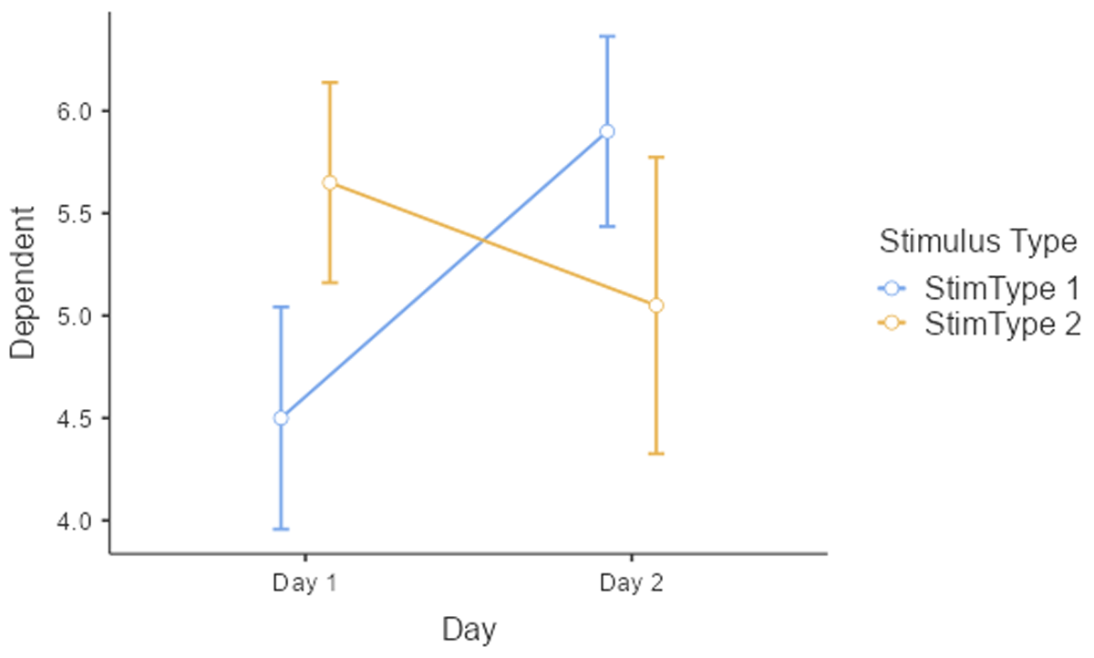
Figure 10
Interaction between Day and Stimulus type. The figure includes the standard errors around the means (based on jamovi).
Table 10
Input for jamovi and R to run a 2 × 2 ANOVA of the data of Table 10, together with the means and the standard deviations of the conditions.
| PARTICIPANT | d1s1 | d1s2 | d2s1 | d2s2 |
|---|---|---|---|---|
| Participant 1 | 3 | 5 | 4 | 2.5 |
| Participant 2 | 6 | 5.5 | 4.5 | 3.5 |
| Participant 3 | 3.5 | 4 | 5.5 | 2.5 |
| Participant 4 | 1.5 | 4.5 | 5.5 | 2.5 |
| Participant 5 | 5 | 8 | 8.5 | 8 |
| Participant 6 | 4.5 | 6 | 7 | 5.5 |
| Participant 7 | 6 | 7 | 5.5 | 6.5 |
| Participant 8 | 4 | 4 | 5 | 4.5 |
| Participant 9 | 4 | 4.5 | 5.5 | 6.5 |
| Participant 10 | 7.5 | 8 | 8 | 8.5 |
| M = | 4.5 | 5.65 | 5.9 | 5.05 |
| SD = | 1.72 | 1.55 | 1.47 | 2.29 |
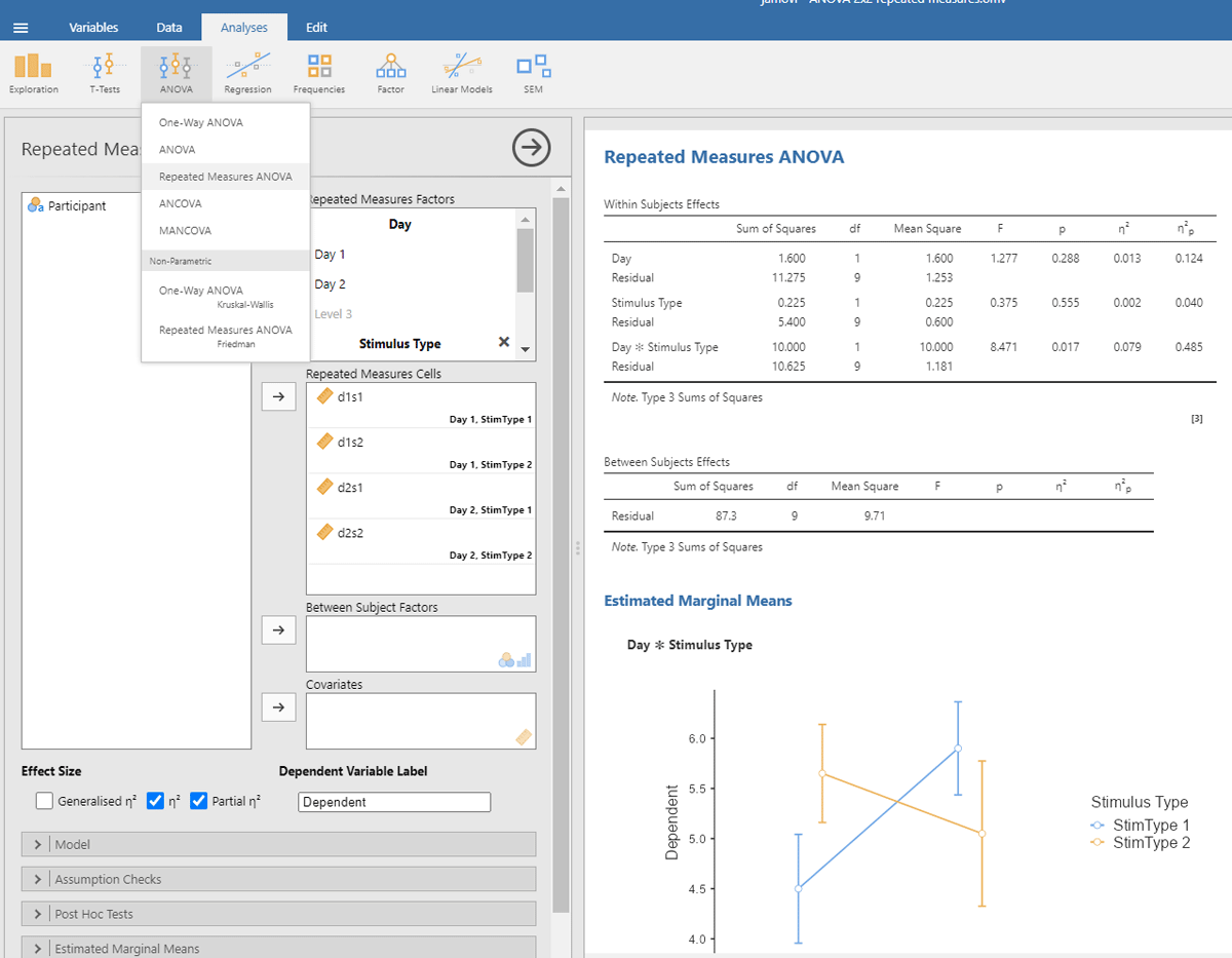
Figure 11
Output jamovi ANOVA 2 × 2 repeated-measures design.
Table 11
Table to show how to center the values of Table 10 for each participant.
| PARTICIPANT | d1s1 | d1s2 | d2s1 | d2s2 | MEAN | d1s1C | d1s2C | d2s1C | d2s2C |
|---|---|---|---|---|---|---|---|---|---|
| Participant 1 | 3 | 5 | 4 | 2.5 | 3.625 | –0.625 | 1.375 | 0.375 | –1.125 |
| Participant 2 | 6 | 5.5 | 4.5 | 3.5 | 4.875 | 1.125 | 0.625 | –0.375 | –1.375 |
| Participant 3 | 3.5 | 4 | 5.5 | 2.5 | 3.875 | –0.375 | 0.125 | 1.625 | –1.375 |
| Participant 4 | 1.5 | 4.5 | 5.5 | 2.5 | 3.5 | –2 | 1 | 2 | –1 |
| Participant 5 | 5 | 8 | 8.5 | 8 | 7.375 | –2.375 | 0.625 | 1.125 | 0.625 |
| Participant 6 | 4.5 | 6 | 7 | 5.5 | 5.75 | –1.25 | 0.25 | 1.25 | 0.25 |
| Participant 7 | 6 | 7 | 5.5 | 6.5 | 6.25 | –0.25 | 0.75 | –0.75 | 0.25 |
| Participant 8 | 4 | 4 | 5 | 4.5 | 4.375 | –0.375 | –0.375 | 0.625 | 0.125 |
| Participant 9 | 4 | 4.5 | 5.5 | 6.5 | 5.125 | –1.125 | –0.625 | 0.375 | 1.375 |
| Participant 10 | 7.5 | 8 | 8 | 8.5 | 8 | –0.5 | 0 | 0 | 0.5 |
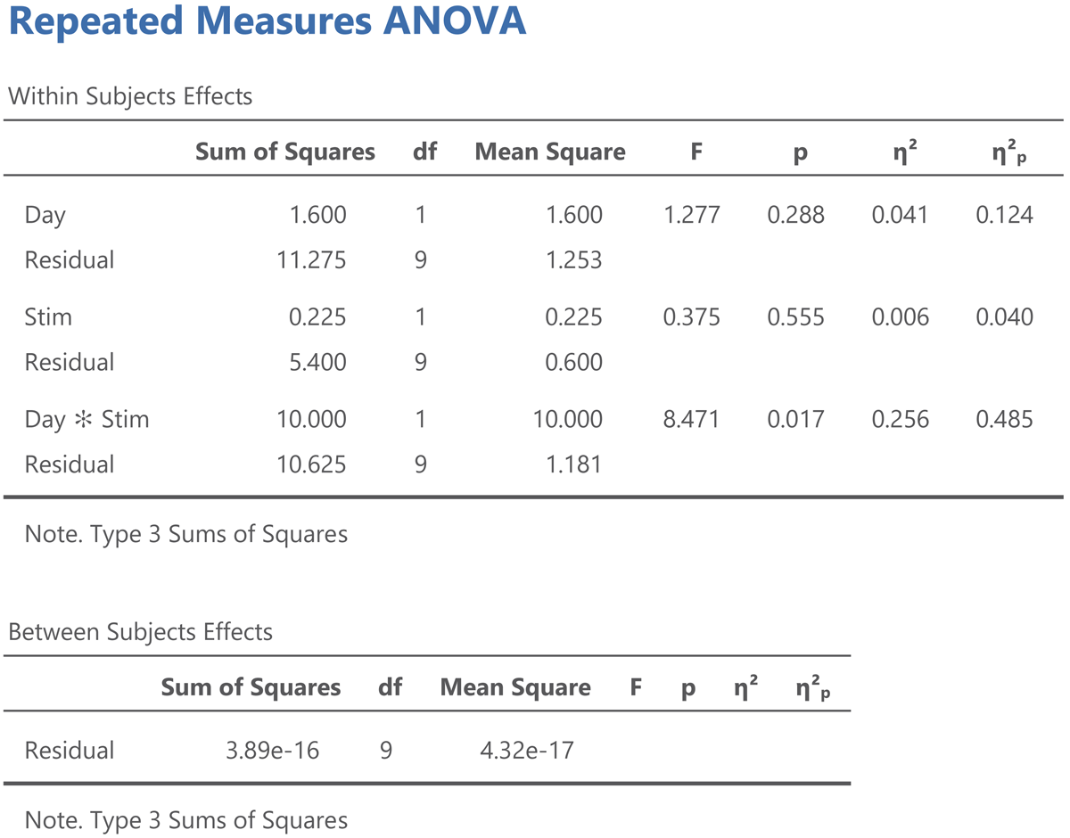
Figure 12
Jamovi output for an ANOVA on the participant centered values from Table 12.
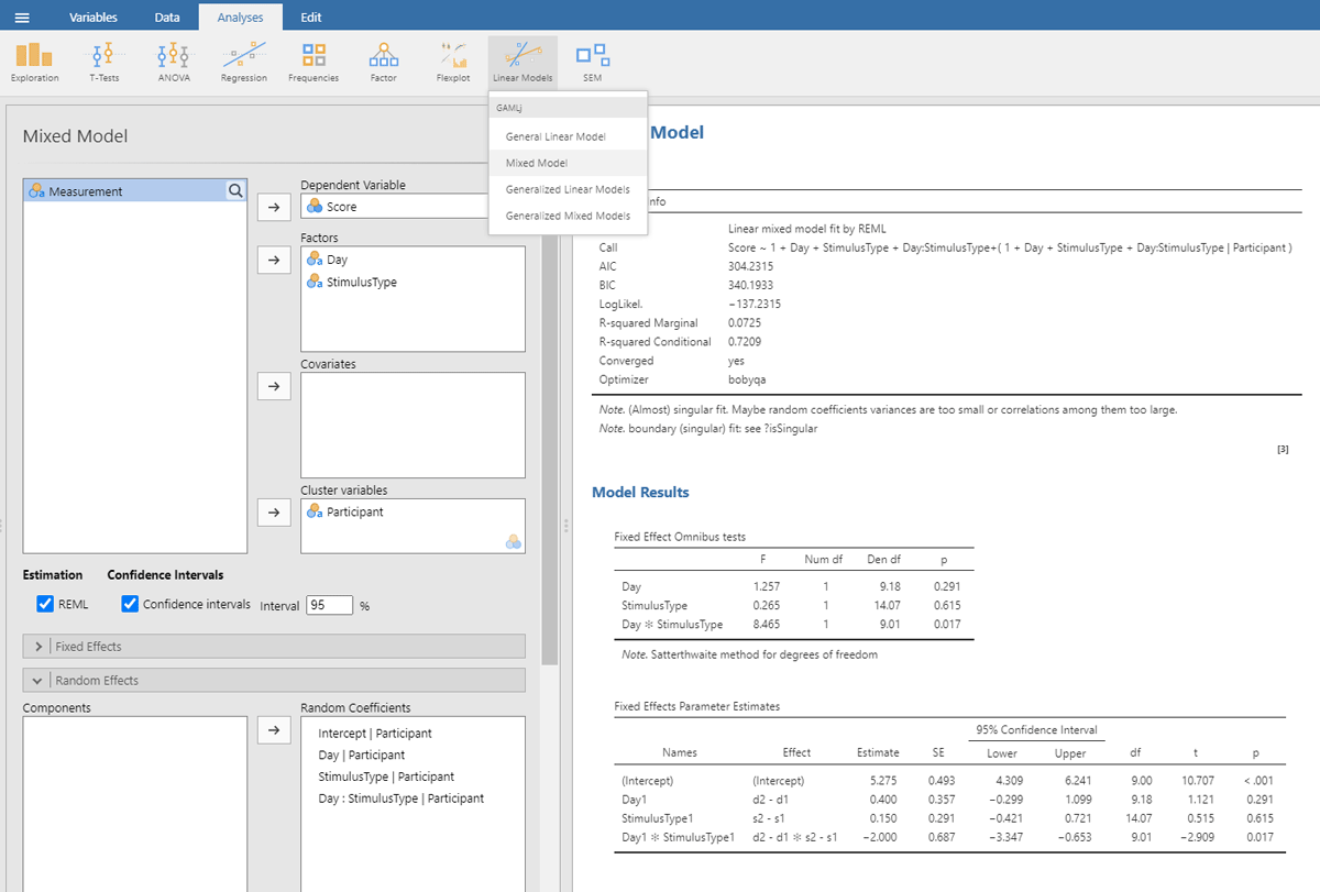
Figure 13
Output jamovi LME analysis 2 × 2 repeated-measures design.
| Fixed Effects Parameter Estimates | ||||||
| NAMES | EFFECT | ESTIMATE | SE | df | t | p |
| (Intercept) | (Intercept) | 5.275 | 0.493 | 9.00 | 10.707 | <.001 |
| Day1 | d2 – d1 | 0.400 | 0.357 | 9.18 | 1.121 | 0.291 |
| StimulusType1 | s2 – s1 | 0.150 | 0.291 | 14.07 | 0.515 | 0.615 |
| Day1 * StimulusType1 | d2 – d1 * s2 – s1 | –2.000 | 0.687 | 9.01 | –2.909 | 0.017 |
| Random Components | ||||
| GROUPS | NAME | SD | VARIANCE | ICC |
| Participant | (Intercept) | 1.511 | 2.283 | 0.665 |
| Day1 | 0.835 | 0.697 | ||
| Stimulus type1 | 0.522 | 0.273 | ||
| Day1 * Stimulus type1 | 1.556 | 2.421 | ||
| Residual | 1.073 | 1.152 | ||
| Note. Number of Obs: 80, groups: Participant 10 | ||||
Table 12
Data from the study of face attractiveness (S1 = stimulus 1, P1 = participant 1, yr18 = 18-year-old, yr75 = 75-year-old). Dependent variable is attractiveness rating on a Likert scale from 1 (unattractive) to 7 (attractive).
| PARTICIPANT | AGE | S1 | S2 | S3 | S4 | S5 | S6 | S7 | S8 | S9 | S10 |
|---|---|---|---|---|---|---|---|---|---|---|---|
| P1 | yr18 | 4 | 3 | 2 | 4 | 2 | 5 | 3 | 5 | 1 | 6 |
| P2 | yr18 | 5 | 4 | 5 | 5 | 4 | 5 | 3 | 5 | 4 | 5 |
| P3 | yr18 | 5 | 3 | 2 | 5 | 2 | 2 | 5 | 5 | 2 | 3 |
| P4 | yr18 | 4 | 3 | 3 | 3 | 1 | 1 | 4 | 5 | 4 | 5 |
| P5 | yr18 | 7 | 2 | 4 | 6 | 2 | 3 | 3 | 4 | 2 | 4 |
| P6 | yr18 | 7 | 5 | 1 | 6 | 2 | 5 | 5 | 5 | 3 | 7 |
| P7 | yr18 | 7 | 3 | 2 | 4 | 1 | 4 | 3 | 5 | 5 | 5 |
| P8 | yr18 | 5 | 4 | 4 | 3 | 3 | 1 | 3 | 4 | 4 | 6 |
| P9 | yr18 | 4 | 4 | 5 | 4 | 2 | 5 | 4 | 5 | 4 | 5 |
| P10 | yr18 | 6 | 3 | 3 | 5 | 2 | 2 | 4 | 5 | 4 | 7 |
| P11 | yr75 | 6 | 2 | 5 | 3 | 1 | 4 | 1 | 3 | 3 | 5 |
| P12 | yr75 | 6 | 1 | 2 | 5 | 3 | 4 | 4 | 1 | 1 | 4 |
| P13 | yr75 | 5 | 2 | 1 | 2 | 3 | 2 | 3 | 1 | 1 | 5 |
| P14 | yr75 | 4 | 3 | 4 | 5 | 2 | 5 | 5 | 3 | 3 | 7 |
| P15 | yr75 | 4 | 1 | 4 | 3 | 1 | 3 | 1 | 1 | 1 | 5 |
| P16 | yr75 | 6 | 3 | 4 | 6 | 2 | 4 | 4 | 1 | 2 | 3 |
| P17 | yr75 | 7 | 3 | 5 | 6 | 4 | 4 | 2 | 2 | 2 | 4 |
| P18 | yr75 | 7 | 5 | 5 | 2 | 2 | 5 | 4 | 4 | 3 | 5 |
| P19 | yr75 | 5 | 3 | 5 | 4 | 2 | 3 | 2 | 1 | 3 | 5 |
| P20 | yr75 | 6 | 1 | 1 | 5 | 2 | 3 | 1 | 1 | 3 | 4 |
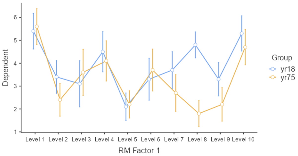
Figure 14
Average ratings of the young and old group per stimulus.
Table 13
Summary table for a related-samples t-test across stimuli.
| STIMULUS | yr18 | yr75 |
|---|---|---|
| S1 | 5.4 | 5.6 |
| S2 | 3.4 | 2.4 |
| S3 | 3.1 | 3.6 |
| S4 | 4.5 | 4.1 |
| S5 | 2.1 | 2.2 |
| S6 | 3.3 | 3.7 |
| S7 | 3.7 | 2.7 |
| S8 | 4.8 | 1.8 |
| S9 | 3.3 | 2.2 |
| S10 | 5.3 | 4.7 |
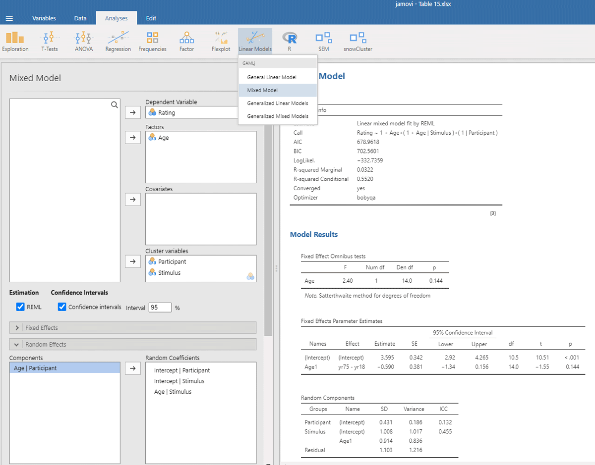
Figure 15
Output jamovi LME analysis face rating study.
Table 14
Data from a study on text reading (language = language of the text, background = whether or not the reader is expected to be familiar with the topic of the text, p1 = participant 1, t1 = text 1). Dependent variable is seconds needed to read a 125 word text.
| LANGUAGE | BACKGROUND | TEXT | p1 | p2 | p3 | p4 | p5 | p6 | p7 | p8 | p9 | p10 | p11 | p12 |
|---|---|---|---|---|---|---|---|---|---|---|---|---|---|---|
| L1 | Yes | t1 | 36 | 31 | 25 | 41 | 25 | 21 | 37 | 31 | 28 | 22 | 30 | 25 |
| L1 | Yes | t2 | 38 | 29 | 32 | 30 | 30 | 37 | 38 | 34 | 36 | 25 | 30 | 32 |
| L1 | Yes | t3 | 38 | 25 | 32 | 46 | 25 | 30 | 42 | 30 | 41 | 22 | 28 | 36 |
| L1 | Yes | t4 | 48 | 24 | 28 | 40 | 28 | 28 | 40 | 26 | 36 | 19 | 40 | 30 |
| L1 | Yes | t5 | 38 | 22 | 28 | 32 | 30 | 35 | 37 | 31 | 38 | 21 | 33 | 24 |
| L1 | No | t6 | 39 | 36 | 40 | 42 | 35 | 30 | 55 | 34 | 34 | 28 | 48 | 42 |
| L1 | No | t7 | 34 | 17 | 35 | 34 | 25 | 19 | 43 | 29 | 30 | 19 | 39 | 43 |
| L1 | No | t8 | 42 | 26 | 36 | 40 | 31 | 31 | 44 | 36 | 31 | 34 | 43 | 30 |
| L1 | No | t9 | 42 | 26 | 35 | 32 | 34 | 25 | 42 | 31 | 39 | 31 | 36 | 40 |
| L1 | No | t10 | 45 | 34 | 36 | 41 | 35 | 28 | 52 | 36 | 40 | 28 | 33 | 34 |
| L2 | Yes | t11 | 34 | 21 | 26 | 30 | 33 | 29 | 39 | 30 | 34 | 30 | 28 | 29 |
| L2 | Yes | t12 | 39 | 24 | 26 | 37 | 27 | 29 | 46 | 31 | 47 | 27 | 33 | 34 |
| L2 | Yes | t13 | 41 | 28 | 25 | 39 | 28 | 35 | 38 | 32 | 43 | 28 | 35 | 23 |
| L2 | Yes | t14 | 32 | 27 | 32 | 44 | 20 | 25 | 42 | 27 | 44 | 18 | 39 | 33 |
| L2 | Yes | t15 | 46 | 22 | 31 | 42 | 33 | 31 | 40 | 34 | 58 | 33 | 32 | 29 |
| L2 | No | t16 | 41 | 27 | 44 | 34 | 38 | 42 | 49 | 45 | 42 | 43 | 51 | 37 |
| L2 | No | t17 | 50 | 39 | 42 | 35 | 34 | 39 | 49 | 42 | 37 | 33 | 43 | 37 |
| L2 | No | t18 | 57 | 37 | 50 | 40 | 46 | 49 | 45 | 38 | 45 | 38 | 45 | 36 |
| L2 | No | t19 | 46 | 32 | 38 | 31 | 37 | 36 | 56 | 33 | 40 | 34 | 38 | 26 |
| L2 | No | t20 | 51 | 36 | 40 | 35 | 40 | 38 | 53 | 27 | 42 | 37 | 40 | 35 |
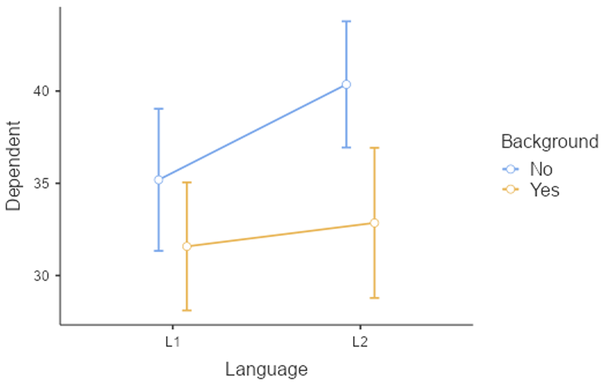
Figure 16
Figure of reading times as a function of Language and Background knowledge.
Table 15
Findings in the analyses by participants and by texts, limited to the ANOVAs.
| ANOVA BY PARTICIPANTS (F1 ANALYSIS) | ANOVA BY TEXTS (F2 ANALYSIS) |
|---|---|
| 2 × 2 analysis with repeated measures | 2 × 2 analysis with between-text variables |
| Main effect Language: F(1,11) = 13.85, p = .003, η² = .061, η²p = .557 | Main effect Language: F(1,16) = 9.45, p = .007, η² = .166, η²p = .371 |
| Main effect Background: F(1,11) = 22.00, p < .001, η² = .181, η²p = .667 | Main effect Background: F(1,16) = 28.09, p < .001, η² = .493, η²p = .637 |
| Interaction: F(1,11) = 5.66, p = .037, η² = .022, η²p = .340 | Interaction: F(1,16) = 3.45, p = .082, η² = .061, η²p = .177 |