
Table 1
Summary of the main hypotheses, models, variables, and effects of interest.
| HYPOTHESIS | CONCEPTUAL MODEL | MODEL AND VARIABLES | EFFECT(S) OF INTEREST | REMARK |
|---|---|---|---|---|
| 1. Compared to the generic masculine form, the internall and feminine masculine form will yield a higher number of women mentioned. | 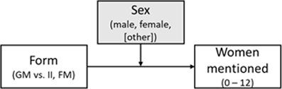 | General linear model (ANOVA); IV: form, moderator: participant sex, DV: women mentionedi; additional multilevel model with Poisson-distributed measures per category nested in participants and labs | Helmert contrast (GM vs. II & FM); Cohen’s d for the mean difference |
|
| 2. Compared to the generic masculine and the control form, the internal-I, feminine masculine, and gender star form will yield a higher number of women mentioned. | 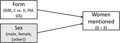 | Multilevel model with Poisson-distributed measures per category nested in participants and labs, IV1: form, IV2: participant sexii, DV: women mentioned | Deviation contrast (GM & C vs II. FM & GS); standardized effect: incident rate ratio |
|
| 3. Higher scores on the perceived base rate (perceived higher proportion of women) are associated with a higher number of women mentioned, when it is controlled for the form effect. | 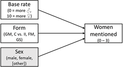 | Multilevel model with Poisson-distributed measures per category (I1) nested in participants (I2), IV1: form, IV2: perceived base rate, DV: women mentioned | Effect of the perceived base rate (level 1) and of the form as in H2 (level 2); standardized effect: incident rate ratio |
|
[i] Note: GM = generic masculine, C = control, II = internal I, FM = feminine-masculine, GS = gender star; i an additional multilevel model will be calculated for Hypothesis 1, ii a language form × sex interaction will also be checked for Hypothesis 2, but effects will be taken from the covariate model; variables in gray boxes are controlled for, but not of primary interest; this table is revised and the original table can be found in Supplemental Materials 3 (https://osf.io/ecpgx).
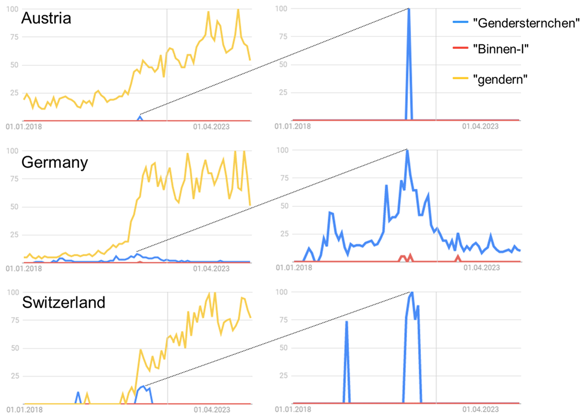
Figure 1
Google searches for ‘gendern’ (using gender-inclusive language in everyday language), ‘Binnen-I’ (internal I) and ‘Gendersternchen’ (gender star) from Jan 2018 to June 2024.
Note: Based on a population of >60 million German users, >7 million Austrian users, and >8 million Swiss users; updated figure and original figure is in Supplemental Materials 3, https://osf.io/ecpgx; searches in percent are standardized on the maximum search per country; diagonal lines across panels connect reference maxima; absolute number of searches is not provided by Google Trends; example search for upper left panel: https://trends.google.de/trends/explore?date=2018-01-012024–05–18&geo=AT&q=Gendersternchen,Binnen-I,gendern.
Table 2
Characteristics of the samples used to test the specific hypotheses.
| LAB | n | GENDER | AGE | HIGHEST LEVEL OF EDUCATION | CHILDHOOD RESIDENCE | NATIONALITY | |||||||||||||
|---|---|---|---|---|---|---|---|---|---|---|---|---|---|---|---|---|---|---|---|
| MEN | WOMEN | DIV. | M (SD); MIN–MAX | NONE | P/S SCHOOL | EXT. S SCHOOL | H/T SCHOOL | UNI. | VILLAGE | CITY | BIG CITY | METROP. | AT | DE | CH | OTHER | NA | ||
| H1 | |||||||||||||||||||
| Bauch* | 62 | 11 | 51 | 0 | 28.65 (10.08); 18–63 | 0 | 0 | 5 | 40 | 17 | 38 | 20 | 3 | 1 | 0 | 61 | 0 | 1 | 0 |
| Beitner* | 83 | 18 | 64 | 1 | 31.13 (9.67); 18–60 | 0 | 0 | 1 | 27 | 55 | 30 | 32 | 21 | 0 | 1 | 82 | 0 | 0 | 0 |
| Brohmer & Hofer | 125 | 70 | 55 | 0 | 35.96 (12.20); 20–71 | 0 | 0 | 1 | 22 | 102 | 69 | 29 | 24 | 3 | 118 | 4 | 0 | 3 | 0 |
| Giuliani* | 68 | 16 | 52 | 0 | 30.68 (11.56); 18–74 | 0 | 2 | 0 | 26 | 40 | 27 | 26 | 10 | 5 | 5 | 27 | 35 | 1 | 0 |
| Gruber | 121 | 31 | 90 | 0 | 25.69 (11.62); 18–73 | 0 | 1 | 1 | 87 | 32 | 65 | 35 | 14 | 7 | 57 | 60 | 0 | 4 | 0 |
| Jauk | 189 | 66 | 122 | 1 | 29.06 (13.85); 18–76 | 0 | 0 | 5 | 101 | 83 | 67 | 56 | 56 | 10 | 1 | 188 | 0 | 0 | 0 |
| Malkoc* | 56 | 28 | 28 | 0 | 30.70 (12.10); 18–65 | 0 | 0 | 0 | 23 | 33 | 35 | 14 | 5 | 2 | 50 | 3 | 0 | 1 | 2 |
| Muees* | 86 | 19 | 66 | 1 | 28.14 (8.83); 18–65 | 0 | 0 | 1 | 36 | 49 | 31 | 21 | 10 | 24 | 70 | 12 | 1 | 2 | 1 |
| Salwender & Berkessel | 217 | 42 | 173 | 2 | 25.37 (6.15); 18–63 | 0 | 0 | 2 | 107 | 108 | 101 | 62 | 40 | 14 | 2 | 210 | 0 | 2 | 3 |
| Wehrt & Otto | 124 | 31 | 93 | 0 | 27.90 (10.56); 18–64 | 0 | 0 | 2 | 76 | 46 | 60 | 49 | 10 | 5 | 1 | 122 | 0 | 1 | 0 |
| ZPID-AT** | 162 | 68 | 93 | 1 | 48.07 (14.28); 19–79 | 0 | 7 | 25 | 87 | 43 | 74 | 36 | 25 | 27 | 151 | 11 | 0 | 0 | 0 |
| ZPID-DE** | 186 | 73 | 112 | 1 | 53.56 (17.00); 18–87 | 0 | 12 | 52 | 68 | 54 | 56 | 76 | 40 | 14 | 1 | 184 | 0 | 1 | 0 |
| Total | 1479 | 473 | 999 | 7 | 34.08 (15.62); 18–87 | 0 | 22 | 95 | 700 | 662 | 653 | 456 | 258 | 112 | 457 | 964 | 36 | 16 | 6 |
| H2 & H3 | |||||||||||||||||||
| Bauch* | 117 | 16 | 101 | 0 | 28.50 (9.74); 18–63 | 0 | 0 | 10 | 85 | 22 | 68 | 43 | 4 | 2 | 0 | 116 | 0 | 1 | 0 |
| Beitner* | 136 | 30 | 104 | 2 | 30.00 (8.52); 18–60 | 0 | 0 | 1 | 40 | 95 | 41 | 52 | 40 | 3 | 1 | 134 | 0 | 1 | 0 |
| Brohmer & Hofer | 224 | 121 | 102 | 1 | 37.32 (12.95); 20–100 | 0 | 0 | 4 | 38 | 182 | 133 | 50 | 37 | 4 | 209 | 11 | 0 | 3 | 1 |
| Giuliani* | 110 | 29 | 81 | 0 | 31.06 (11.68); 18–74 | 0 | 2 | 0 | 45 | 63 | 42 | 40 | 16 | 12 | 9 | 42 | 55 | 2 | 2 |
| Gruber | 227 | 56 | 171 | 0 | 25.08 (9.94); 18–73 | 0 | 2 | 1 | 167 | 57 | 117 | 64 | 33 | 13 | 99 | 123 | 0 | 5 | 0 |
| Jauk | 345 | 111 | 232 | 2 | 29.05 (14.19); 18–76 | 1 | 1 | 7 | 200 | 136 | 131 | 105 | 98 | 11 | 1 | 344 | 0 | 0 | 0 |
| Malkoc* | 111 | 54 | 57 | 0 | 31.05 (12.26); 18–71 | 0 | 0 | 0 | 44 | 67 | 65 | 32 | 10 | 4 | 99 | 8 | 0 | 2 | 2 |
| Muees* | 162 | 37 | 124 | 1 | 28.42 (9.41); 18–68 | 0 | 0 | 1 | 65 | 96 | 66 | 45 | 14 | 37 | 131 | 23 | 1 | 5 | 2 |
| Salwender & Berkessel | 375 | 79 | 293 | 3 | 25.90 (7.43); 18–79 | 0 | 0 | 5 | 190 | 180 | 166 | 120 | 67 | 22 | 2 | 367 | 0 | 2 | 4 |
| Wehrt & Otto | 232 | 52 | 177 | 3 | 27.85 (10.63); 18–68 | 0 | 0 | 3 | 146 | 83 | 103 | 92 | 27 | 10 | 1 | 228 | 0 | 2 | 1 |
| ZPID-AT** | 324 | 129 | 193 | 2 | 48.13 (14.39); 19–79 | 0 | 17 | 44 | 182 | 81 | 145 | 72 | 49 | 58 | 307 | 17 | 0 | 0 | 0 |
| ZPID-DE** | 334 | 139 | 192 | 3 | 53.89 (16.61); 18–87 | 1 | 26 | 94 | 115 | 98 | 90 | 138 | 80 | 26 | 2 | 330 | 0 | 2 | 0 |
| Total | 2697 | 853 | 1827 | 17 | 34.38 (15.79); 18–100 | 2 | 48 | 170 | 1317 | 1160 | 1167 | 853 | 475 | 202 | 861 | 1743 | 56 | 25 | 12 |
[i] Note: Div. = Diverse; P/S school = primary or secondary school; Ext. S school = extended secondary school (‘Real-’ or ‘Mittelschule’); H/T school = high school diploma or trade school; Univ. = university degree; Metrop. = metropolis; AT = Austria; DE = Germany; CH = Switzerland; Other = other nationality (often double citizenship with either German or Austrian included); NA = response not provided.
* Labs that could not reach the anticipated samples of n = 200 to 250; ** Additional samples to achieve the anticipated sample size.
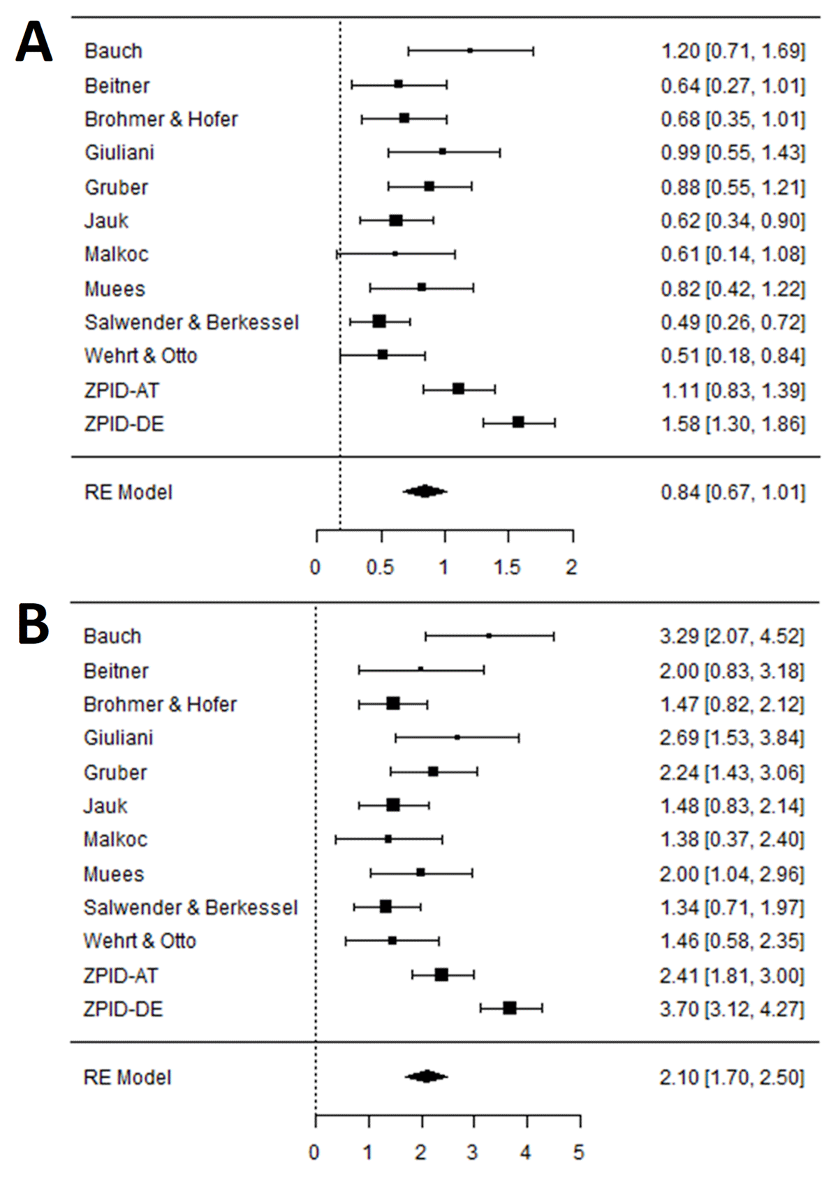
Figure 2
Forest Plots of the Main Contrast of Interest in Hypothesis 1 (Generic-Masculine vs. Internal-I and Feminine-Masculine Form).
Note: N = 1479. Panel A shows the contrast expressed in the Cohen’s d metric. The vertical line represents our smallest effect size of interest (d = 0.18). Panel B shows the mean difference in the original metric (number of women mentioned; 0–12). The vertical line represents an effect of 0. Squares represent effects per lab with error bars being 90% confidence intervals (for one-sided testing). Diamonds are meta-analytic random effects.
Table 3
Mean number of women mentioned per sex, category, and group.
| SEX | CATEGORY | CONTROL (n = 594) | GENERIC M. (n = 550) | INTERNAL-I (n = 473) | FEM.-MASC. (n = 551) | GENDER S. (n = 529) | |||||
|---|---|---|---|---|---|---|---|---|---|---|---|
| M | SD | M | SD | M | SD | M | SD | M | SD | ||
| Male | Actor+ | 0.66 | 0.69 | 0.50 | 0.71 | 1.09 | 1.11 | 0.80 | 0.85 | 0.80 | 0.86 |
| Politician | 0.80 | 0.71 | 0.68 | 0.62 | 1.21 | 0.94 | 0.82 | 0.64 | 0.85 | 0.77 | |
| Singer | 0.79 | 0.88 | 0.69 | 0.91 | 1.84 | 1.08 | 1.01 | 0.83 | 1.50 | 1.03 | |
| Athlete | 0.15 | 0.37 | 0.16 | 0.42 | 0.74 | 1.08 | 0.26 | 0.47 | 0.33 | 0.64 | |
| TV host | 0.54 | 0.64 | 0.57 | 0.76 | 1.05 | 1.04 | 0.69 | 0.76 | 0.72 | 0.82 | |
| Writer+ | 0.52 | 0.66 | 0.40 | 0.63 | 0.96 | 0.98 | 0.64 | 0.73 | 0.67 | 0.76 | |
| Female | Actor+ | 1.02 | 0.82 | 0.84 | 0.86 | 1.49 | 0.97 | 1.18 | 0.82 | 1.18 | 0.92 |
| Politician | 1.01 | 0.73 | 0.85 | 0.71 | 1.50 | 0.97 | 1.07 | 0.65 | 1.14 | 0.76 | |
| Singer | 1.22 | 0.91 | 0.98 | 1.02 | 2.31 | 0.87 | 1.60 | 0.91 | 1.90 | 0.95 | |
| Athlete | 0.45 | 0.66 | 0.30 | 0.60 | 1.08 | 1.11 | 0.53 | 0.72 | 0.62 | 0.89 | |
| TV host | 0.78 | 0.75 | 0.81 | 0.82 | 1.32 | 1.02 | 1.04 | 0.85 | 1.05 | 0.88 | |
| Writer+ | 1.18 | 0.87 | 0.99 | 0.89 | 1.58 | 0.97 | 1.24 | 0.88 | 1.35 | 0.92 | |
[i] Note: N = 2,697. SD = standard deviation. + = category introduced for the extended replication. Possible range: 0–3.
Table 4
Ratios of differences in the number of named women between conditions (pairwise comparisons).
| CONTRAST | RATIO | SE | z-RATIO | p |
|---|---|---|---|---|
| C vs. GM | 1.19 | 0.04 | 5.50 | <.001 |
| C vs. II | 0.59 | 0.02 | –18.38 | <.001 |
| C vs. FM | 0.84 | 0.02 | –5.79 | <.001 |
| C vs. G* | 0.77 | 0.02 | –9.02 | <.001 |
| GM vs. II | 0.49 | 0.02 | –23.01 | <.001 |
| GM vs. FM | 0.71 | 0.02 | –11.04 | <.001 |
| GM vs. G* | 0.64 | 0.02 | –14.11 | <.001 |
| II vs. FM | 1.44 | 0.04 | 12.66 | <.001 |
| II vs. G* | 1.31 | 0.04 | 9.38 | <.001 |
| FM vs. G* | 0.91 | 0.03 | –3.27 | .011 |
[i] Note: N = 2697. C = control condition. GM = generic masculine. II = internal-I. FM = feminine-masculine. G* = gender star. p-values are Bonferroni-corrected (adjusted for 10 tests). Tests were performed on the log scale. Values above 1 indicate a higher number of women named in the left compared to the right condition (e.g, in the first row, more people were named in the C than in the GM condition).
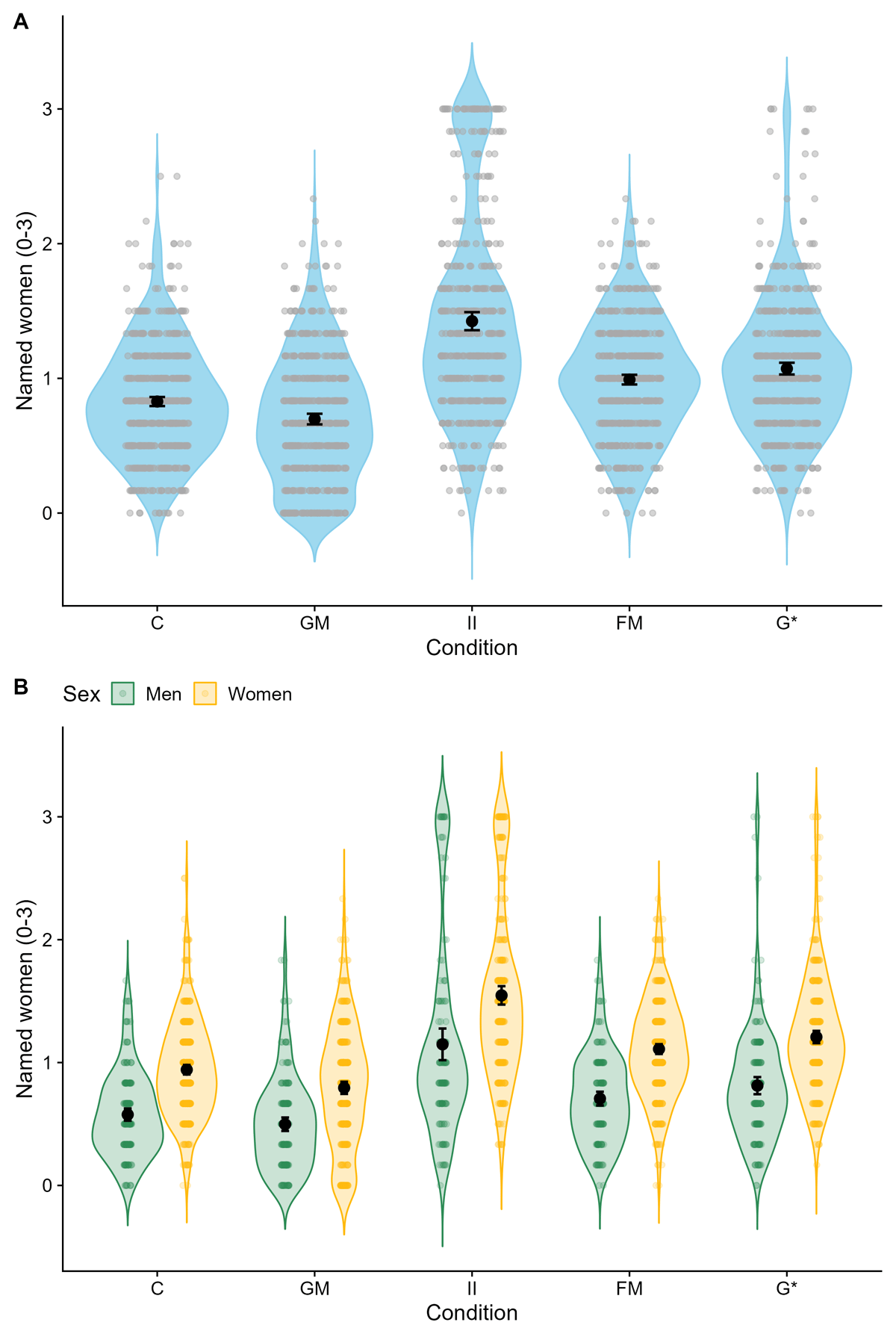
Figure 3
Violin plots showing the number of women named per condition (A) and per condition and sex (B).
Note: N = 2,697. Black dots indicate means and 95% confidence intervals. Colorful dots are participant-level data. C = control condition. GM = generic masculine. II = internal-I. FM = feminine-masculine. G* = gender star.
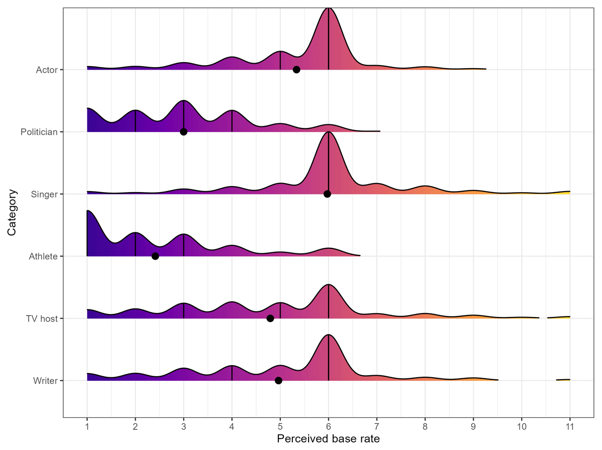
Figure 4
Ridgeline plots showing the perceived base rate per category.
Note: N = 2,697. Black dots indicate means and 95% confidence intervals (not visible here, due to precise estimation). Black horizontal lines indicate quartiles. The scale ranged from 1 (‘Men are much more present than women’) to 11 (‘Women are much more present than men’).