
1. Introduction
Climate change is resulting in increasing average temperatures and more frequent heatwaves (IPCC 2023), with warming occurring faster at higher latitudes due to polar amplification caused by increased melting of snow and ice and other feedback mechanisms (Mikkonen et al. 2015; Rantanen et al. 2022). In Finland, annual average temperatures have increased by almost 2°C since 1901 (Ruosteenoja & Räisänen 2021). This warming is resulting in milder winters, with recent anomalies of 2.5°C (2015), 5.0°C (2020) and 1.4°C (2023) above the 1991–2020 average Helsinki winter temperatures of –2.6°C. Summers are also becoming hotter, with 2018, 2021 and 2022 averaging 1.5, 2.1 and 1.3°C above the 1991–2020 average summertime temperature of 16.3°C in Helsinki, respectively (Finnish Meteorological Institute 2024). Heatwave events are becoming more frequent, long and intense (Kim et al. 2018; Mikkonen et al. 2015).
Temperatures may be modified by the urban heat island (UHI) effect, the phenomenon whereby urban centres are hotter than surrounding rural areas, caused by the presence of materials such as concrete and asphalt which absorb and retain heat during the day due to their thermal and surface radiative properties; low levels of evapotranspiration from soil moisture, vegetation and water features; anthropogenic heat emissions; and differences in morphology that impact airflow and solar radiation (Oke et al. 2017). In Finland, prior research has indicated a maximum UHI intensity (or the difference between temperatures within a city and the surrounding rural area) of up to 14°C in Helsinki and around 10–12°C in Turku (Drebs et al. 2023).
Elevated UHI temperatures have implications for energy consumption. In cold climate UHIs, increased air and ground temperatures can be a net benefit in terms of energy consumption (Brozovsky et al. 2021) by reducing building space heating demands and increasing potential to use local heat energy from groundwater (Arola & Korkka-Niemi 2014). In the Nordic countries, the number of homes with heat pumps is rapidly increasing; given that heat pump efficiency reduces at lower outdoor temperatures, the UHI may also lead to increased heating efficiency in many homes. On the other hand, the UHI can lead to increases in energy use for summertime space cooling (Brozovsky et al. 2021), particularly for homes designed for cold rather than heat (Taylor et al. 2023).
The associations between temperature and health are well-documented. In cold Nordic climates, temperature-related mortality is dominated by cold effects (Masselot et al. 2023; Oudin Åström et al. 2018; Ruuhela et al. 2018), and in Finland annual average excess deaths from cold are estimated at around 1450, and from heat at around 45 (Masselot et al. 2023). However, in Finland, excess mortality increases slowly below optimal temperatures and more rapidly above optimal temperatures, indicting a better adaptation to cold than heat (Tobías et al. 2021). While the UHI may provide a protective effect for cold-related mortality (Macintyre et al. 2021), mortality rates during four intense heatwaves (2003, 2010, 2014 and 2018) were around 2.5 times higher in Helsinki than the surrounding area (Ruuhela et al. 2020), potentially due to increased UHI temperatures. Certain population groups are more vulnerable to non-optimal temperatures, such as older people and the chronically ill (Kollanus et al. 2021; Suulamo et al. 2024).
There is a need to characterise the UHI to understand the potential benefits and mitigate any risks or disbenefits in colder and less heat-adapted cities. Various approaches can evaluate urban climate. Many studies rely on remotely sensed land surface temperature (LST); however, LST can be a poor predictor of urban-canopy air temperature (Chakraborty et al. 2022; Du et al. 2024; Venter et al. 2021). The UHI can be modelled using computationally expensive urban climate models to examine air temperatures for defined time periods, e.g. scenarios with the presence and absence of urban surfaces, or to investigate the expected impact of different urban climate adaptation scenarios (Brousse et al. 2024b; Suomi et al. 2024). Researcher-deployed networks of weather stations can evaluate UHI, often alongside LST, although the number of possible sensors to deploy is limited (Alvi et al. 2022; Bassett et al. 2016; Suomi & Käyhkö 2012). Finally, urban temperatures can be estimated by spatially interpolating air temperatures from station measurements (Aalto et al. 2016), although with likely high levels of uncertainty with increasing distances from stations.
The recent emergence of personal weather stations (PWS) has provided opportunities to use crowd-sourced meteorological data in urban climate research (Meier et al. 2017; Muller et al. 2015; Steeneveld et al. 2011; de Vos et al. 2020; Wolters & Brandsma 2012). These citizen-provided data offer increased coverage of measured air temperature data across many urban environments. PWS data have been used, for example, to supplement official meteorological data (de Vos et al. 2017; O’Hara et al. 2023), examine the role of landcover on air temperatures (Brousse et al. 2022; Du et al. 2024; Fenner et al. 2017; Potgieter et al. 2021; Taylor et al. 2024; Varentsov et al. 2021), model air temperatures (Venter et al. 2020; Vulova et al. 2020; Zumwald et al. 2021), validate and bias-correct urban climate simulations (Blunn et al. 2024; Brousse et al. 2023; Hammerberg et al. 2018), or as input to building physics models (Benjamin et al. 2021). Due to their lower costs and non-research deployment, PWS data have greater uncertainty than official automatic weather stations (AWS), and measurements from individual PWS are noisy (Brousse et al. 2023). However, methods have been developed to help clear data and remove erroneous stations and measurements (Fenner et al. 2021). While deployment of AWS or research weather stations may be strategically planned, PWS may be unequally distributed due to, for example, low populations or socio-economic differences (Brousse et al. 2024a). These so-called ‘sensor deserts’ can influence the amount and quality of data available across different communities and environments, limiting the generalisation of urban climate studies, empowerment of communities and reducing climate adaptation potential.
Studies into cold-climate and high-latitude UHIs are relatively scarce (Varentsov et al. 2023) despite rapidly changing climates and their implications for energy and exposure to non-optimal temperatures. This paper leverages a dense network of PWS in Finland to examine sensor coverage, characterise UHI intensity and heterogeneity, and study its implications for energy and extreme temperatures in four cold climate metropolitan areas (Helsinki, Vantaa, Espoo and Tampere). To achieve this, hourly PWS and AWS temperature data for municipal administrative areas and surroundings are obtained for the period January 2018–December 2023. PWS were spatially linked to local climate zones (LCZs), urban–rural classifications, and gridded built environment and socio-economic information. The distribution of PWS across communities and landcover type was assessed to evaluate proximity to populations and identify where, and for whom, temperature data are available. Hourly data were then used to examine temperature distributions across LCZs and UHI intensity at different seasons, times of day and reference temperatures. Finally, urban–rural differences in heating degree-days (HDD), cooling degree-days (CDD) and population exposures to extreme temperatures were calculated.
2. Methods
The study period was from 1 January 2018 to 31 December 2023, selected due to the growing availability of PWS data during this time. Helsinki, Vantaa, Espoo and Tampere are the four largest municipalities in Finland by population, each with a warm-summer, humid-continental climate (Koppen Dfb), but with Tampere bordering on the subarctic climate zone (Dfc). Helsinki, Espoo and Vantaa are part of the same metropolitan area, and together form the capital region.
2.1 PWS Data
PWS information was obtained from Netatmo stations operating during the study period, within domains defined by a bounding box surrounding a 50-km buffer of the administrative boundaries of each municipality; for adjoining municipalities, these buffers overlap. For each station within the domains, PWS station ID and coordinates were obtained using the Patatmo Python module that uses the Netatmo API (https://dev.netatmo.com/).
For each PWS, hourly near-surface air temperatures were downloaded for the study period using Patatmo. Temperature data were cleaned with the R package CrowdQC+ (Fenner et al. 2021), which includes several steps for quality control of PWS data. First, a height correction was applied to each PWS by spatially joining terrain height from a 10-m resolution digital elevation model of Finland (National Land Survey of Finland 2019). Temperature data were then cleaned using the following steps:
M1: removal of hourly measurements from stations located at the same coordinates, and assumed to be duplicates.
M2: removal of outlier hourly temperatures, as determined by their z-score.
M3: stations where more than 20% of the measurements in the month were removed in the previous steps, and therefore assumed to be unreliable.
M4: removal of temperature measurements which were uncorrelated to the median temperature of neighbouring PWS stations (Pearson r < 0.9) and therefore assumed to be indoors.
Finally, if a sensor had a day with more than 3 h of absent data, this day was removed.
Hourly reference temperatures were taken from Finnish Meteorological Institute AWS at Helsinki-Vantaa Airport (Helsinki, Espoo and Vantaa) and Härmälä (Tampere). Cleaned hourly PWS temperatures were linked to the corresponding AWS reference temperatures for each location and converted from UTC to local time. Based on the time and date, air temperature measurements were classified according to season, daytime (07.00–19.00 hours) or night-time (20.00–06.00 hours), and during daylight or dark hours (calculated based on their longitude and latitude using the suncalc package).
2.2 Location analysis
PWS were then classified according to their locations to examine coverage and location bias. They were filtered only to include those within the 50-km buffer of the administrative city boundaries of each urban area.
Spatial linkages to environment data were performed to evaluate the environments where PWS were located. Spatial joins to urban–rural classifications from the Finnish Environment Institute (SYKE 2018) were used to classify PWS as being urban (inner urban areas, outer urban areas) or rural (local rural centres, rural areas close to urban areas, rural heartland areas and sparsely populated rural areas) irrespective of administrative boundaries and to provide a rural reference for urban temperatures. Urban PWS were those in areas classified as urban within municipal boundaries, while rural PWS were in areas classified as rural within municipal boundaries and the surrounding buffer. A spatial join linked PWS to YKR (Monitoring System of Spatial Structure and Urban Form) 250-m gridded data on built environment characteristics (sparse small homes, small homes, apartments or cottages) (SYKE & Statistics Finland 2023a) and to LCZs at 100-m resolution (Demuzere et al. 2019).
Spatial linkages to socio-demographic data were performed to evaluate the communities covered by PWS data. YKR 250-m grid resolution socio-demographic data (population, unemployment and number of pensioners) (SYKE & Statistics Finland 2023b) were spatially joined to PWS. Unemployment was used as a proxy for socio-economic status to evaluate biases in coverage, while pensioner population was used to identify whether PWS are represented in locations with high numbers of heat-vulnerable residents. Socio-economic data were classified into quantiles within administrative areas (by grid cell count), while grid cells where data were withheld due to low population counts were left unclassified.
Descriptive analyses were used to assess the representativeness of the PWS locations, including the count of sensors and sensor-hours (or hours of cleaned temperature data). The numbers of PWS that fell into different urban–rural or built environment typologies and LCZs were calculated. The distribution of PWS stations across the different socio-economic quantiles was calculated for the municipalities. The distance from each municipal YKR grid cell to its nearest AWS or PWS was calculated and used to examine population-weighted average distance to different station types.
2.3 Temperature analysis
2.3.1 UHI intensity and land cover
Hourly temperatures, linked to land classifications, were then analysed to characterise urban temperatures. Descriptive statistics were used to summarise urban and rural PWS temperatures for different seasons. UHI intensity was calculated as the hourly differences between average rural (non-water and within buffer region) and the corresponding average urban (non-water and within administrative boundaries) temperatures. Density plots were used to illustrate the distribution of hourly UHI intensity for daytime, night-time, season, and daylight or dark hours. This was repeated, comparing rural average PWS temperatures with the hottest urban PWS (90th percentile within administrative boundaries) to illustrate the maximal hourly difference.
To examine how urban–rural temperature differences may change with reference temperatures, the PWS station anomaly (or the difference between daily average temperature at a PWS station compared with the reference AWS temperature) was plotted dependent on the reference temperature for urban and rural locations. Anomalies were also calculated for the different LCZs within municipalities to examine spatial heterogeneity.
2.3.2 Extreme temperature exposures
Epidemiological studies often examine excess mortality on cold or hot days, where such days are identified using thresholds based on daily average temperature percentiles, e.g. 5th and 10th percentiles (Sohail et al. 2023) for cold and 90th and 95th percentiles (Sohail et al. 2020) for heat. These thresholds were calculated from long-term (2001–17) temperatures from reference AWS and used to define hot or cold days where temperatures can be harmful for population health. On days when reference stations were above or below thresholds, the daily average, daytime average maximum and night-time average minimum temperatures were calculated for urban, rural and reference stations. Annual average counts of the number of days that thresholds were exceeded were also calculated.
2.3.3 Space heating and cooling
Implications for space heating and cooling were calculated for urban and rural PWS using HDD and CDD, respectively. HDD were calculated when daily average temperature were below a threshold of 12°C (until December) or 10°C (after December), while CDD were calculated from May to September inclusive for days when the average temperature exceeded 18°C (Pirinen et al. 2024).
3. Results
3.1 PWS Locations
The locations of PWS and AWS for the different study locations, LCZs, and urban–rural classifications are shown in Figure 1. Results indicate a dense coverage of PWS locations. Most stations are concentrated in urban centres, but with reasonable coverage in surrounding rural areas. In total, 997 PWS stations were analysed, growing from 160 in early 2018, with numbers of PWS broadly reflecting the populations of the different metropolitan areas (Table 1).
Table 1
Summary statistics from personal weather stations (PWS) and reference automatic weather stations (AWS).
| HELSINKI | ESPOO | VANTAA | TAMPERE | ||
|---|---|---|---|---|---|
| PWS count | |||||
| Within administrative boundaries | 202 | 137 | 75 | 78 | |
| Urban | 199 | 129 | 72 | 72 | |
| Peri-urban | 2 | 0 | 3 | 0 | |
| Rural | 1 | 8 | 0 | 6 | |
| Within buffera | 677 | 719 | 695 | 274 | |
| Urban | 509 | 517 | 517 | 136 | |
| Peri-urban | 118 | 119 | 119 | 24 | |
| Rural | 50 | 83 | 59 | 114 | |
| Average distance (nearest) (km) | Reference | 3.1 | 5.4 | 5.9 | 4.7 |
| PWS | 0.26 | 0.35 | 0.36 | 0.52 | |
| Seasons | |||||
| Winter daily average (°C) | Reference | –2.9 | –3.7 | ||
| Urban PWS | –1.7 | –2.0 | –2.4 | –3.5 | |
| Rural PWS | –2.8 | –2.7 | –3.0 | –3.8 | |
| Spring daily average (°C) | Reference | 4.9 | 4.9 | ||
| Urban PWS | 6.1 | 5.4 | 5.7 | 5.5 | |
| Rural PWS | 4.9 | 5.0 | 4.9 | 4.9 | |
| Summer daily average (°C) | Reference | 17.7 | 17.1 | ||
| Urban PWS | 18.9 | 18.6 | 18.6 | 17.9 | |
| Rural PWS | 17.8 | 17.8 | 17.8 | 17.3 | |
| Autumn daily average (°C) | Reference | 6.8 | 6.0 | ||
| Urban PWS | 7.9 | 7.5 | 7.1 | 6.3 | |
| Rural PWS | 6.8 | 6.9 | 6.6 | 5.9 | |
[i] Note: aDue to shared administrative borders, these contain overlapping PWS.
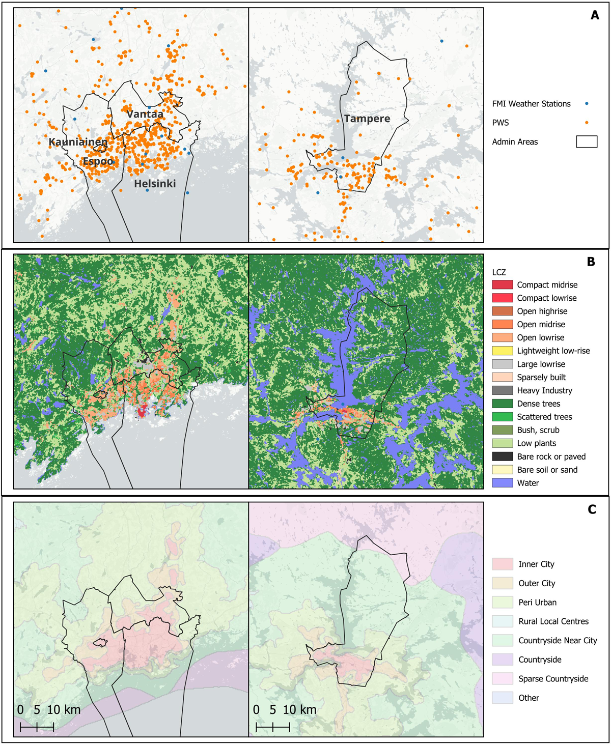
Figure 1
(a) Locations of personal weather stations (PWS) and official stations for the different study areas, as well as the administrative boundaries; (b) their local climate zone (LCZ) classifications; and (c) their urban–rural classifications.
Most municipal PWS were in areas classified as open mid-rise (19% of land area in Helsinki, 2.2% in Espoo, 5.4% in Vantaa and 2.4% in Tampere) or open low-rise (15.4% of land area in Helsinki, 16.3% in Espoo, 14.3% in Vantaa and 2.8% in Tampere), according to LCZ categories. Compact high-rise was not present in any study area, while open high-rise was present in Tampere, but only 1000 m2 and with no PWS present.
Distributions of PWS across different socio-demographic characteristics are shown in Figure 2, including station counts and cleaned sensor-hours since 2018. The number of sensor-hours broadly reflects the counts of sensors. There are greater numbers of sensors in areas with higher population density in all locations. Areas with the most and least unemployment tended to have the fewest PWS, while patterns across pensioner quantiles varied by city.
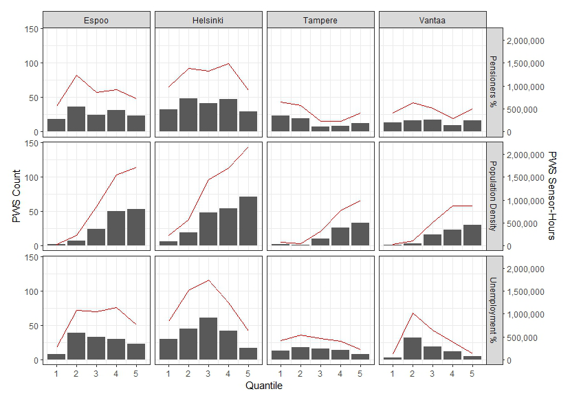
Figure 2
Counts of personal weather stations (PWS) by 250-m grid cell according to the percentage of pensioners in the population, population density and unemployment rates, where 1 is the lowest and 5 is the highest.
Note: Counts are shown in bars; sensor-hours are shown with a red line.
Analysis across built-environment classifications indicates most PWS were in areas defined by small homes (55%), followed by apartments (18%) and cottages (14%). On average, a resident in Helsinki lives 3.1 km from an AWS, with 5.4 km in Espoo, 5.9 km in Vantaa and 4.7 km in Tampere. Proximity to PWS is much higher, with the population-average distance to PWS in Helsinki of 257 m, in Espoo of 345 m, in Vantaa of 356 m and in Tampere of 515 m. In Helsinki, for example, around 8% of the population lives within 1 km of an official station, but nearly 100% within 1 km of a PWS, and 50% of the population within 200 m of their nearest PWS.
3.2 Air temperatures
Summary statistics in Table 1 show the average daily temperatures for reference stations, urban PWS and rural PWS for different seasons. Reference stations are closer in temperature to rural PWS, with urban PWS showing a UHI effect. The distributions of hourly urban–rural temperature differences are shown in Figure 3. The greatest difference between hourly average urban and rural temperatures was seen in the largest city, Helsinki (1.2°C, interquartile range (IQR) = 0.6–1.2°C), followed by Espoo (0.8, 0.4–1.2°C), Vantaa (0.7, 0.4–1.1°C) and Tampere (0.5, 0.1–0.8°C). Differences in average urban and rural temperatures were greater during spring and summer than in autumn and winter. Average differences are also greater during day (07.00–20.00) and night (21.00–06.00) hours than during daylight and dark hours, which vary seasonally due to the high latitude. Maximum differences in urban and rural average temperatures were 6.4°C (Helsinki), 5.3°C (Espoo), 4.7°C (Vantaa) and 4.2°C (Tampere). Over a 24-h period, on average, the greatest daily UHI intensity in Espoo occurred around 04.00 hours (1.1°C), Helsinki around 05.00 hours (1.5°C), Tampere at 02.00 hours (0.7°C) and Vantaa at 16.00 hours (0.8°C). Urban cool islands were present, occurring most commonly during summer (11% of hours) and least frequently in autumn (8% of hours), and predominantly during daytime.
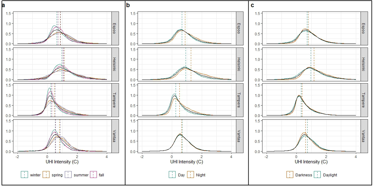
Figure 3
Density plots of the distributions of hourly urban heat island (UHI) intensity for (a) seasons; (b) day (07.00–20.00 hours) and night (21.00–06.00 hours); and (c) daylight or dark hours.
Note: Black lines show the density for all groups as a reference; vertical lines show the median for each distribution.
Figure S1 in the Appendix shows the same analysis for the hottest 10% of PWS within the urban areas. The average differences between rural areas and the hottest urban areas were 2.7°C (IQR = 1.7–3.4°C) for Helsinki, 1.9°C (IQR = 1.1–2.6°C) for Espoo, 1.7°C (IQR = 0.9–2.2°C) for Tampere and 1.8°C (IQR = 1.0–2.4°C) for Vantaa. Helsinki experienced a maximum intensity of 10.7°C, Espoo of 9.0°C, Vantaa of 8.7°C and Tampere of 8.1°C. Differences between median temperatures are more apparent when using 90th percentile urban temperatures for different seasons, and for daylight/darkness, indicating a potential influence of solar radiation on urban heating and potentially PWS exposure to direct sunlight.
Temperatures for urban and rural areas are shown relative to reference AWS temperatures in Figure 4, with the temperature anomaly describing daily average temperature differences. In all municipalities, urban temperatures are typically higher than rural temperatures, with the hottest 10% of rural PWS similar to the median urban PWS. Urban temperatures have a greater average difference to the reference AWS and rural PWS on hot and cold days. Reference AWS more closely reflect the median rural temperatures than urban temperatures, potentially because official AWS tend to be sited in less built-up areas.
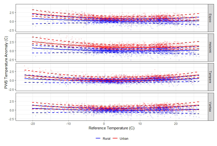
Figure 4
Variation of the daily average temperature anomalies (difference between personal weather station (PWS) temperature and reference daily average temperature) according to reference automatic weather station (AWS) temperature for urban and rural locations.
Note: Solid lines indicate the median anomaly; dashed lines show its 10th and 90th percentiles.
The temperature distributions for different LCZs, and the count of PWS stations in each LCZ, are shown in Figure 5 for the administrative areas and the surrounding buffers; Figures S2 and S3 in the Appendix show the same analyses for PWS within municipal boundaries for day/night and different seasons. PWS counts across LCZs in the municipalities reflect differences in urban structures, with fewer in natural or sparsely built areas, and more in LCZs typical of residential areas. Temperature anomalies tended to be highest in large low-rise areas (the exception being Tampere, likely due to a small sample size), compact mid-rise and open low-rise, and lowest in more natural LCZs, except in cases with low sample sizes. Anomalies tended to be higher at night and are at their greatest during summer.
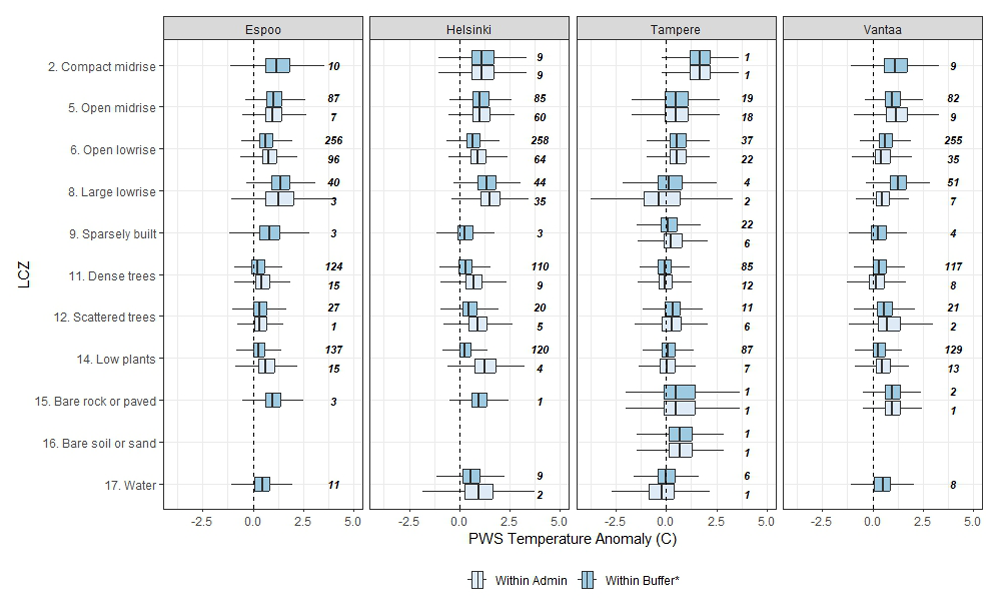
Figure 5
Personal weather station (PWS) temperature anomaly (average difference between the PWS temperatures and reference temperatures during a day) for each municipality and local climate zone (LCZ) present.
Note: Counts of PWS in each LCZ are also shown.
*Within buffers include overlapping PWS stations for Helsinki, Espoo and Vantaa.
3.2.1 Degree-days and temperature extremes
Table 2 shows the daily average, average daytime maximum and average night-time minimum temperatures, when temperatures are outside the thresholds, as well as the annual average number of days temperatures are outside the thresholds during the seven-year period of the study. Urban PWS both exceed heat thresholds more frequently and are hotter than rural or reference AWS. For example, the 10th percentile is exceeded by, on average, 15 more days than the reference AWS in Helsinki. On days above heat thresholds, urban–rural differences tend to be greatest for night-time minimum temperatures compared with daytime maximum.
Table 2
For reference stations and urban and rural personal weather stations (PWS), temperatures when daily average automatic weather stations (AWS) temperatures are above or below temperature percentiles, heating degree-days (HDD) and cooling degree-days (CDD).
| HELSINKI | ESPOO | VANTAA | TAMPERE | ||
|---|---|---|---|---|---|
| Above 90th percentile | |||||
| Average 24-h mean (°C) (count of days) | Reference | 20.8 (36) | 20.1 (39) | ||
| Urban PWS | 21.8 (51) | 21.6 (48) | 21.6 (46) | 21.0 (47) | |
| Rural PWS | 20.7 (38) | 20.7 (38) | 20.7 (37) | 20.2 (40) | |
| Average daytime maximum (°C) | Reference | 25.5 | 25.1 | ||
| Urban PWS | 27.0 | 26.9 | 27.5 | 26.4 | |
| Rural PWS | 25.9 | 25.8 | 25.8 | 25.9 | |
| Average night minimum (°C) | Reference | 15.1 | 13.9 | ||
| Urban PWS | 17.3 | 16.5 | 15.9 | 16.1 | |
| Rural PWS | 15.4 | 15.4 | 15.4 | 14.6 | |
| Days above 95th percentile | |||||
| Average 24-h mean (°C) (count of days) | Reference | 22.2 (21) | 21.7 (21) | ||
| Urban PWS | 23.3 (28) | 23.0 (25) | 23.1 (26) | 22.7 (29) | |
| Rural PWS | 22.1 (20) | 22.0 (21) | 22.0 (20) | 21.8 (22) | |
| Average daytime maximum (°C) | Reference | 27.0 | 27.0 | ||
| Urban PWS | 28.5 | 28.3 | 29.0 | 28.3 | |
| Rural PWS | 27.4 | 27.3 | 27.3 | 27.8 | |
| Average night minimum (°C) | Reference | 16.4 | 15.2 | ||
| Urban PWS | 18.6 | 17.7 | 17.2 | 17.6 | |
| Rural PWS | 16.6 | 16.6 | 16.6 | 15.9 | |
| Days below 10th percentile | |||||
| Average 24-h mean (°C) (count of days) | Reference | –9.4 (27) | –10.2 (28) | ||
| Urban PWS | –7.4 (18) | –7.9 (20) | –8.6 (24) | –9.4 (25) | |
| Rural PWS | –9.1 (27) | –9.0 (27) | –9.3 (28) | –10.1 (28) | |
| Average daytime maximum (°C) | Reference | –6.6 | –7.3 | ||
| Urban PWS | –4.9 | –5.2 | –5.8 | –6.9 | |
| Rural PWS | –6.4 | –6.3 | –6.6 | –7.3 | |
| Average night minimum (°C) | Reference | –13.0 | –13.8 | ||
| Urban PWS | –10.0 | –10.7 | –11.7 | –12.0 | |
| Rural PWS | –12.1 | –12.0 | –12.3 | –13.1 | |
| Days below 5th percentile | |||||
| Average 24-h mean (°C) (count of days) | Reference | –12.6 (12) | –13.9 (11) | ||
| Urban PWS | –10.3 (7) | –10.9 (8) | –11.8 (10) | –12.6 (9) | |
| Rural PWS | –12.1 (11) | –12.1 (10) | –12.4 (11) | –13.7 (11) | |
| Average daytime maximum (°C) | Reference | –9.5 | –9.9 | ||
| Urban PWS | –7.6 | –8.0 | –8.6 | –9.3 | |
| Rural PWS | –9.1 | –9.0 | –9.4 | –10.1 | |
| Average night minimum (°C) | Reference | –16.3 | –18.1 | ||
| Urban PWS | –12.9 | –13.7 | –14.9 | –15.6 | |
| Rural PWS | –15.3 | –15.3 | –15.5 | –17.2 | |
| Energy | |||||
| Annual average HDD | Urban PWS | 2,910 | 2,989 | 3,063 | 3,199 |
| Rural PWS | 3,191 | 3,183 | 3,229 | 3,311 | |
| Annual average CDD | Urban PWS | 156 | 140 | 141 | 123 |
| Rural PWS | 107 | 108 | 108 | 94 | |
[i] Note: Counts of the annual average number of days when thresholds are exceeded are also shown.
Fewer days below cold thresholds were observed in urban PWS relative to rural PWS or reference AWS. Comparatively large urban–rural differences can be observed for night-time minimum temperatures and daytime maximum temperatures compared with the daily average. Temperatures for days below the cold thresholds are also higher for urban PWS compared with rural PWS or reference AWS, and with comparatively fewer days below the thresholds. Relative to the period 2000–17, the number of days exceeding the heat threshold is slightly higher than expected for reference AWS, and notably less for cold days, suggesting some warming relative to this baseline. The relative increase in hot days due to the UHI tended to be larger than the relative decrease in cool days for the same percentiles.
The number of HDD and CDD in urban and rural PWS is also shown in Table 2. Relative to rural PWS, urban PWS experienced an average of 281 fewer HDD/year over the period 2018–23 in Helsinki, 194 in Espoo, 166 in Vantaa and 112 in Tampere. The increased urban temperatures led to a corresponding, but relatively smaller, increase in the numbers of CDD: 49 in Helsinki, 32 in Espoo, 33 in Vantaa and 29 in Tampere.
4. Discussion
Data for 997 PWS stations in and around Tampere, Helsinki, Espoo and Vantaa were used to examine the coverage and representativeness of PWS, quantify the UHI effects, and calculate the potential implications for energy and health.
Researcher-led deployment of sensors allows for locations to be selected strategically, while in this case PWS locations are based on community actions. Studies (Brousse et al. 2024a) have shown areas with PWS deserts in the UK, and therefore less temperature coverage, for example. The present results indicate greater coverage of PWS in more densely populated areas, as expected. Greater numbers of PWS are generally seen in areas with the lowest and the highest unemployment, but with no other consistent biases according to income or the number of pensioners. The lower number of PWS in areas with higher unemployment levels (e.g. in Espoo and Vantaa) indicate that such communities may be underrepresented when using PWS data; conversely, in all municipalities except Tampere, there was relatively good PWS coverage in areas with a higher percentage of pensioners, suggesting good coverage in areas with heat-vulnerable residents. Analysis with population grid density indicates that PWS can provide measured temperature data for residential locations, proximate to the majority of the metropolitan population.
While the PWS offer increased density of coverage, the present analyses do indicate a bias in landcover type which may impact the results. The majority of PWS are in areas defined by small housing or apartments (e.g. open low-rise and open mid-rise), with relatively few in the compact mid-rise areas which characterise dense commercial urban centres in Finland and where the UHI may be greatest. The relatively high number of PWS in rural areas with cottages means there are a large amount of data against which urban temperatures can be referenced to estimate UHI intensity. Cottages are likely often located near lakes and may be subject to cooling from water evaporation, although the present analyses exclude all LCZ classified as ‘water’.
While location biases of PWS add an important context to the results, the ranges and maximum values (90th percentile) for UHI intensity are similar to those of previous studies for Helsinki (Drebs et al. 2023). Clear differences in UHI intensity were seen by season, with spring and summer showing greater average UHI intensities than autumn or winter in all locations. While peak UHI values tended to be higher during the night in all municipalities except Vantaa, distributions of UHI intensity were similar. Compared with day and night hours, relatively larger differences for maximal (90th percentile) intensities were instead seen across daylight and dark hours, indicating the importance of solar radiation and long summer days on UHI formation—and potentially measurement error.
Urban–rural differences are greatest at low- and high-reference AWS temperatures, suggesting that UHI intensity increases at temperature extremes. Temperatures from reference AWS are closer to those from rural PWS, indicating that studies that rely on these measurements for temperature exposures may miss the UHI effect. Rural PWS exhibit similar temperatures to reference AWS, increasing confidence in the data quality control. Larger municipalities had more LCZs with relatively high temperature anomalies, and temperature anomalies tended to be greatest in LCZs with a greater built fraction, during the night and during the summer. The residential bias for PWS, and different urban structures across municipalities, mean that some LCZs classifications (e.g. natural areas) can lack data, leading to highly variable anomaly distributions.
While PWS temperatures will be subject to greater measurement error, their density and proximity to populations can help identify locations where air temperatures are greater or lesser that official AWS measurements, and capture temperature extremes that could otherwise be missed when relying on AWS. As an example, the maximum hourly temperature at the reference AWS for Helsinki was 32.4°C, which occurred on 28 July 2019. Maximum temperatures for the same day were 32.6°C at the AWS in Kaisaniemi, in Helsinki city centre, while the 90th percentile urban PWS maximum temperature in Helsinki was 36.3°C. Therefore, the hottest PWS were 3.7°C higher than official records for that day.
Greater UHI intensities on very cold and very hot days have implications for public health. Results indicate reduced exposure to cold temperatures and days but also increasing exposure to high temperatures and a larger increase in the number of hot days compared with reduction in cold. Relative to the baseline, the study period exhibited more hot days and fewer cold days, with the UHI exacerbating this further. As relative mortality increases more rapidly at high rather than low temperatures in Finland (Tobías et al. 2021), this indicates a growing risk from heat. However, there is also some evidence that populations living in hotter areas can be adapted to these conditions (Milojevic et al. 2016), and long-term acclimatisation may occur (Arbuthnott et al. 2016). Reduced exposure to cold may also benefit population health. Decreases in excess winter mortality peaks have been observed during the last two decades in Finland (Suulamo et al. 2024), which may be in part attributable to influenza vaccinations. While the risk of mortality increases rapidly with hotter days, days below the minimum mortality temperature of 14°C (Ruuhela et al. 2018) are more common. Future work could apply temperature-mortality functions to UHI temperatures in order to quantify the overall health implications of the UHI (Macintyre et al. 2021).
Against this health context, there are potential benefits for energy. Elevated urban temperatures mean a reduction in HDD four to six times larger than the increase in CDD, suggesting a net benefit for building energy consumption. Energy spent on active cooling can be reduced, in part, through better design and passive cooling solutions, particularly important given heat from air-conditioning can increase UHI temperatures (Brousse et al. 2024b), energy consumption and, depending on energy supply, greenhouse gas emissions. A simplistic method for calculating heating and cooling demand has been used. A recent study in Finland indicates that overheating (indoor temperatures >27°C) occurs even on days with average temperatures of 19°C (Farahani et al. 2024), meaning for buildings prone to overheating, cooling may be required at temperatures below the CDD thresholds calculated in this study.
4.1 Strengths and weaknesses
The application of large amounts of temperature data and dense coverage of PWS is a strength of this study. PWS networks offer a significant increase in the number of air temperature sensors deployed compared with previous studies in Finland (Drebs et al. 2023). The number of stations included in the study is comparably high, with around 335 stations per million population in the municipalities studied, versus 56 per million in a previous study over a similar time period in London, UK (Taylor et al. 2024). The study also uses data over a relatively long period, allowing for long-term averages to be calculated. Other crowd-sourced weather data providers, such as those from Weather Underground (Wunderground) which could have provided additional PWS data coverage, have not been included.
The analysis of sensor coverage examines the representativeness and generalisability of PWS data. The analysis itself is limited to unemployment (used here as a proxy for deprivation), population density, number of pensioners and types of housing. Unemployment is a crude indicator of deprivation. Future analyses could, for example, examine combinations of indicators such as education, health and living environment. Small-level gridded data provide high-spatial-resolution population data, but with confidentiality-related missing data leading to biases towards areas with higher population densities. The high-resolution grid data were selected due to their ability to capture local variations in populations; however, future analysis could examine the effects for additional socio-economic variables available for larger areas.
A limitation of PWS is their accuracy relative to official meteorological stations. This includes instrumental errors due to lower accuracy devices compared with official stations, as well as deployment errors that may occur due to issues such as placement (e.g. potentially close to a source of radiative heat, in direct solar radiation or where they may get wet). Instrumental errors will be reduced, as all PWS are from the same manufacturer. To minimise measurement errors, data-cleaning methods were used to remove outliers, unreliable stations and those likely to be indoors. However, anomaly differences during daylight/dark hours suggest potential impacts of solar radiation on measurements.
The biased coverage of PWS will influence calculated UHI intensity in two ways. First, the rural references for UHI intensity are PWS in surrounding rural areas, and the trends and amplitude of UHI intensity will be sensitive to these stations (Liu et al. 2023). Second, the urban comparator is the average urban PWS temperature as well as those in the top 10%. However, the analyses of PWS locations show that they are predominantly in residential areas, with fewer in dense commercial urban areas, meaning true intensity may be underestimated.
4.2 Implications for policy
Analyses show an extensive and growing availability of PWS data in Finland, which offers significant research potential for evaluating urban climates. These can include, for example, examining heat exposure variations across different urban landcovers (Brousse et al. 2022; Du et al. 2024; Fenner et al. 2017; Potgieter et al. 2021; Taylor et al. 2024; Varentsov et al. 2021), health impact calculations for heat exposure (Taylor et al. 2024), refined estimates of local weather for building simulations (Benjamin et al. 2021) and to correct weather models (Brousse et al. 2023; Hammerberg et al. 2018). Policies and action plans can help protect residents from the risks of extreme heat, but will be most effective if locations where exposure is greatest and populations are most vulnerable are identified (Cheng et al. 2021). While the lack of PWS in dense commercial centres means that the maximum UHI intensity may be underestimated, high coverage in residential areas means good data coverage where people live.
While PWS offer a greater coverage density than AWS, inconsistent distributions of sensors across neighbourhoods means that certain areas may have climate data that are less certain or of lower quality, with implications for research conclusions. There were inconsistent biases across municipalities, with no obvious indication that those with low income, the unemployed or the elderly are underrepresented. However, to increase citizen engagement in urban climate science, climate adaptation and empowerment, PWS may be located by official bodies at, for example, community centres or public buildings in underrepresented areas.
Differences in UHI intensity by season and according to reference temperatures indicate that the UHI can exacerbate heat exposures during hot weather, but potentially provide space heating energy benefits that outweigh cooling costs. There is an increasing need to adapt housing and urban environments to heat as part of wider adaptation strategies, but energy implications should be considered. Further research should investigate whether seasonal or dynamic measures (e.g. deciduous trees, passive or active building cooling) are more appropriate than static measures (e.g. cool surfaces) for reducing extreme heat without potential energy or cold disbenefits in the Finnish context. Future research could extend the analyses conducted to examine thermal comfort differences.
5. Conclusions
Personal weather stations (PWS) was used to examine the urban heat islands (UHI) effect in the Finnish municipalities of Helsinki, Vantaa, Espoo and Tampere. Analysis of PWS locations indicates that they are primarily in residential areas, with greater coverage in areas with higher population densities, but with inconsistent patterns across socio-economic groups. Results of the temperature analyses indicate an average UHI intensity of 1.2°C (interquartile range (IQR) = 0.6–1.2°C) for Helsinki, 0.8°C (IQR = 0.4–1.2°C) for Espoo, 0.7°C (IQR = 0.4–1.1°C) for Vantaa and 0.5°C (IQR = 0.1–0.8°C) for Tampere, with clear seasonal effects. UHI intensities appear to be greatest at low and high temperatures, indicating that the UHI can exacerbate summer heat exposures during hot weather, but may offer benefits for reduced heating demand during cold weather. PWS offer increasing spatial coverage of urban climate data, and the number of operating stations in Finland indicates significant potential for future research. However, understanding the implications of location biases is necessary when interpreting the results.
Appendices
Appendix
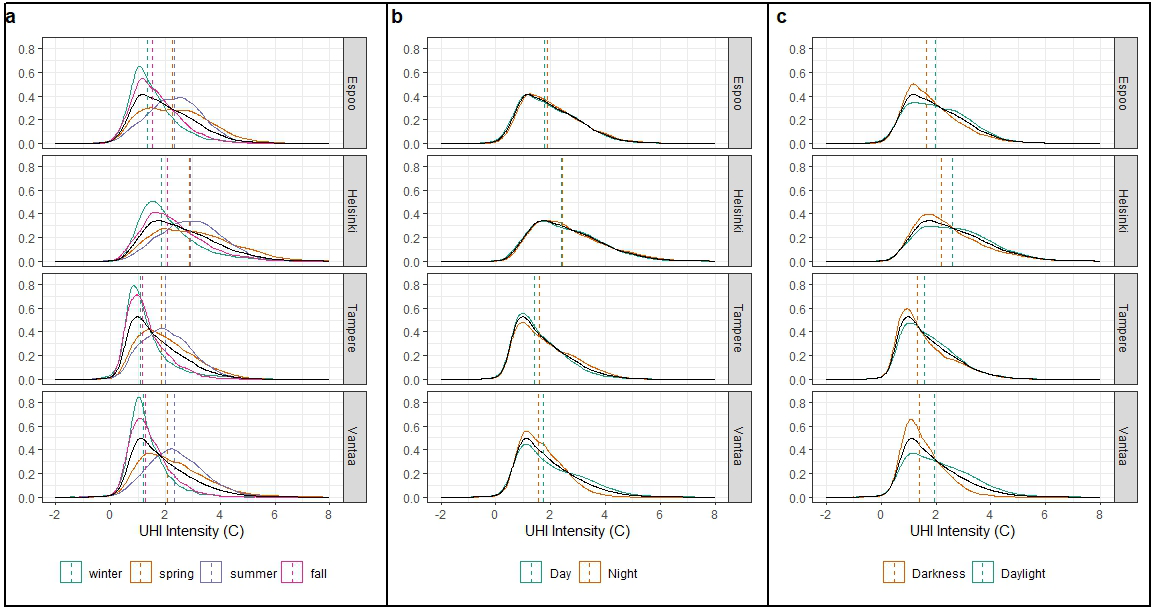
Figure S1
Density plots of the distributions of hourly urban heat island (UHI) intensity (90th percentile urban temperatures) for (a) seasons; (b) day (07.00–20.00 hours) and night (21.00–06.00 hours); and (c) daylight or dark hours.
Note: Black lines show the density for all groups as a reference; vertical lines show the median for each distribution.
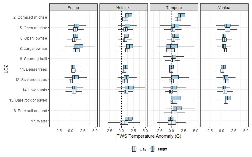
Figure S2
Personal weather station (PWS) temperature anomaly (average difference between daily PWS temperatures and reference temperatures) for each municipality and local climate zone (LCZ) present by day and night for PWS within administrative boundaries.
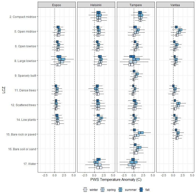
Figure S3
Personal weather station (PWS) temperature anomaly (average difference between daily PWS temperatures and reference temperatures) for each municipality and local climate zone (LCZ) present by day and night for PWS within administrative boundaries
Competing interests
The authors have no competing interests to declare.
Data accessibility
The data are available from Netatmo (https://dev.netatmo.com/). YKR data are available under licence from SYKE in Finland. Local climate zone (LCZ) and postcode data are public datasets.