
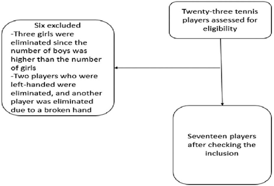
Figure 1
The study participant recruitment flowchart.
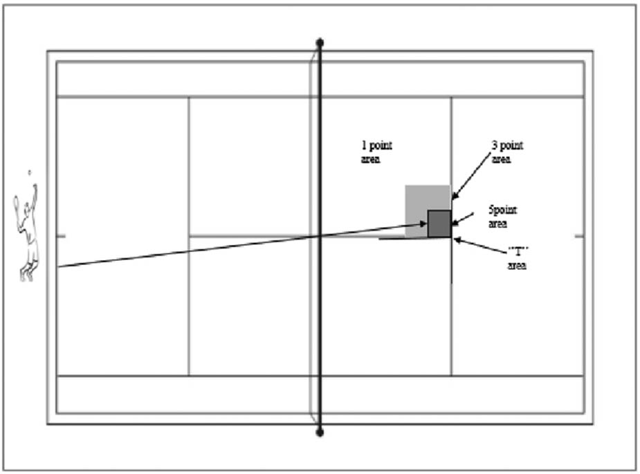
Figure 2
Scoring zones in the serve box.
Table 1
Interaction between conditions and points areas
| Source | Correction | df | Mean square | F | Sig. | Partial eta squared | ε |
|---|---|---|---|---|---|---|---|
| Point area | Greenhouse-Geisser | 1.228 | 1187.745 | 274.756 | 0.001 | 0.945 | 0.614 |
| Condition | Greenhouse-Geisser | 1.414 | 52.050 | 85.612 | 0.001 | 0.843 | 0.707 |
| Point area × Condition | Greenhouse-Geisser | 2.514 | 23.094 | 7.077 | 0.001 | 0.307 | 0.629 |
Greenhouse-Geisser correction was applied due to violation of sphericity (ε = 0.614 for point area; ε = 0.707 for condition; ε = 0.629 for Point area × Condition). η 2 p = partial eta squared. n = 17 per condition.
Table 2
Point area pairwise comparison
| Point Area | Mean Diff. | Std. error Diff. | Sig.bonf | Effect size | |
|---|---|---|---|---|---|
| Point area 5 | Point area 3 | −0.078 | 0.150 | 0.608 | 0.063 |
| Point area 5 | Point area 1 | −6.588 | 0.395 | 0.001 | 2.025 |
| Point area 3 | Point area 1 | −6.51 | 0.366 | 0.001 | 2.156 |
Pairwise comparisons with Bonferroni correction. n = 17 per condition. *p < 0.001 significant effect.
Table 3
Conditions pairwise comparison
| Condition | Mean Diff. | Std. error Diff. | Sig.bonf | Effect size | |
|---|---|---|---|---|---|
| CC | VMC1 | −1.118 | 0.162 | 0.001 | 1.679 |
| CC | VMC2 | −1.667 | 0.131 | 0.001 | 3.087 |
| VMC1 | VMC2 | −0.549 | 0.085 | 0.001 | 1.558 |
CC = control condition; VMC1 = video modelling condition 1 (single exposure); VMC2 = video modelling condition 2 (repeated exposure). Pairwise comparisons with Bonferroni correction. n = 17 per condition. *p < 0.05 significant effect.
Table 4
ANOVA results for successful serve, ball speed, and ball impact across conditions
| Correction | df | Mean square | F | Sig. | Partial eta squared | ε | |
|---|---|---|---|---|---|---|---|
| Succeful_Service | Greenhouse-Geisser | 1.414 | 156.149 | 85.612 | 0.001 | 0.843 | 0.707 |
| Ball_Speed | Sphericity assumed | 2 | 1.938 | 1.652 | 0.208 | 0.094 | 1.000 |
| Ball_Impact | Sphericity assumed | 2 | 103.767 | 70.288 | 0.001 | 0.815 | 1.000 |
Greenhouse-Geisser correction was applied for successful serve (ε = 0.707). Sphericity was assumed for ball speed and ball impact (ε = 1.000). η 2 p = partial eta squared. n = 17 per condition.
Table 5
Pairwise comparisons for successful serve, ball speed, and ball impact across conditions
| Measure | Condition | Mean Diff. | Std. error Diff. | Sig.bonf | Effect size | |
|---|---|---|---|---|---|---|
| Succeful_Service | 1 | 2 | −3.353 | 0.485 | 0.001 | 1.678 |
| 1 | 3 | −5 | 0.393 | 0.001 | 3.086 | |
| 2 | 3 | −1.647 | 0,256 | 0.001 | 1.558 | |
| Ball_Speed | 1 | 2 | 0.671 | 0.404 | 0.116 | 0.403 |
| 1 | 3 | 0.404 | 0.357 | 0.275 | 0.274 | |
| 2 | 3 | −0.267 | 0.352 | 0.458 | 0.184 | |
| Ball_Impact | 1 | 2 | −3.244 | 0.481 | 0.001 | 1.636 |
| 1 | 3 | −4.85 | 0.443 | 0.001 | 2.656 | |
| 2 | 3 | −1.606 | 0.306 | 0.001 | 1.273 |
Pairwise comparisons with Bonferroni correction. CC = control condition; VMC1 = video modelling condition 1; VMC2 = video modelling condition 2. *p < 0.001 significant effect.
Table 6
ANOVA results for condition, test, and their interaction for point area 1
| Source | Correction | df | Mean square | F | Sig. | Partial eta squared | ε |
|---|---|---|---|---|---|---|---|
| Condition | Sphericity assumed | 2 | 189.987 | 55.402 | 0.001 | 0.776 | 1.000 |
| Test | Greenhouse-Geisser | 1.362 | 224.276 | 33.049 | 0.001 | 0.674 | 0.454 |
| Condition × Test | Greenhouse-Geisser | 3.029 | 58.299 | 25.399 | 0.001 | 0.614 | 0.505 |
Greenhouse-Geisser correction was applied for Test (ε = 0.454) and Condition × Test (ε = 0.505). Sphericity was assumed for Condition (ε = 1.000). η 2 p = partial eta squared. n = 17 per condition.
Table 7
Pairwise comparisons between conditions for point area 1
| Condition | Mean Diff. | Std. Error Diff. | Sig.bonf | Effect size | |
|---|---|---|---|---|---|
| CC | VMC1 | −2.099 | 0.372 | 0.001 | 1.370 |
| CC | VMC2 | −3.303 | 0.319 | 0.001 | 2.509 |
| VMC1 | VMC2 | −1.204 | 0.250 | 0.001 | 1.168 |
Pairwise comparisons with Bonferroni correction. CC = control condition; VMC1 = video modelling condition 1; VMC2 = video modelling condition 2. *p < 0.001 significant effect.
Table 8
Pairwise comparisons between tests for point area 1
| Test | Mean Diff. | Std. error Diff. | Sig.bonf | Effect size | |
|---|---|---|---|---|---|
| Point area 1 | SS | −1.529 | 0.154 | 0.001 | 2.407 |
| Point area 1 | BS | 1.65 | 0.499 | 0.004 | 0.801 |
| Point area 1 | BI | −1.076 | 0.253 | 0.001 | 1.033 |
| SS | BS | 3.179 | 0.471 | 0.001 | 1.637 |
| SS | BI | 0.454 | 0.181 | 0.023 | 0.608 |
| BS | BI | −2.726 | 0.365 | 0.001 | 1.809 |
Pairwise comparisons with Bonferroni correction. SS = Successful Serve; BS = Ball Speed; BI = Ball Impact. *p < 0.05 significant effect.
Table 9
ANOVA results for condition, test, and their interaction for point area 3
| Source | Correction | df | Mean square | F | Sig. | Partial eta squared | ε |
|---|---|---|---|---|---|---|---|
| Condition | Sphericity Assumed | 2 | 106.964 | 53.134 | 0.001 | 0.769 | 1.000 |
| Test | Greenhouse-Geisser | 1.904 | 1095.228 | 211.774 | 0.001 | 0.930 | 0.635 |
| Condition × Test | Greenhouse-Geisser | 2.683 | 82.093 | 41.187 | 0.001 | 0.720 | 0.447 |
Greenhouse-Geisser correction was applied for Test (ε = 0.635) and Condition × Test (ε = 0.447). Sphericity was assumed for Condition (ε = 1.000). η 2 p = partial eta squared. n = 17 per condition.
Table 10
Pairwise comparisons between conditions for point area 3
| Condition | Mean Diff. | Std. error Diff. | Sig.bonf | Effect size | |
|---|---|---|---|---|---|
| CC | VMC1 | −1.57 | 0.267 | 0.001 | 1.424 |
| CC | VMC2 | −2.479 | 0.271 | 0.001 | 2.220 |
| VMC1 | VMC2 | −0.91 | 0.181 | 0.001 | 1.219 |
Pairwise comparisons with Bonferroni correction. CC = control condition; VMC1 = video modelling condition 1; VMC2 = video modelling condition 2. *p < 0.001 significant effect.
Table 11
Pairwise comparisons between tests for point area 3
| Test | Mean Diff. | Std. error Diff. | Sig.bonf | Effect size | |
|---|---|---|---|---|---|
| Point area 3 | SS | −8.039 | 0.284 | 0.001 | 3.430 |
| Point area3 | BS | −4.86 | 0.423 | 0.001 | 2.784 |
| Point area3 | BI | −7.586 | 0.352 | 0.001 | 2.611 |
| SS | BS | 3.179 | 0.471 | 0.001 | 1.637 |
| SS | BI | 0.454 | 0.181 | 0.023 | 0.608 |
| BS | BI | −2.726 | 0.365 | 0.001 | 1.809 |
Pairwise comparisons with Bonferroni correction. SS = Successful Serve; BS = Ball Speed; BI = Ball Impact. *p < 0.05 significant effect.
Table 12
ANOVA results for condition, test, and their interaction for point area 5
| Source | df | Mean square | F | Sig. | Partial eta squared | ε | |
|---|---|---|---|---|---|---|---|
| Condition | Sphericity assumed | 2 | 113.366 | 65.551 | 0.001 | 0.804 | 1.000 |
| Test | Greenhouse-Geisser | 1.998 | 1064.442 | 206.675 | 0.001 | 0.928 | 0.666 |
| Condition × Test | Greenhouse-Geisser | 2.991 | 70.423 | 34.816 | 0.001 | 0.685 | 0.499 |
Greenhouse-Geisser correction was applied for Test (ε = 0.666) and Condition × Test (ε = 0.499). Sphericity was assumed for Condition (ε = 1.000). η 2 p = partial eta squared. n = 17 per condition.
Table 13
Pairwise comparisons between conditions for point area 5
| Condition | Mean Diff. | Std. error Diff. | Sig.bonf | Effect size | |
|---|---|---|---|---|---|
| CC | VMC1 | −1.614 | 0.254 | 0.001 | 1.542 |
| CC | VMC2 | −2.553 | 0.247 | 0.001 | 2.503 |
| VMC1 | VMC2 | −0.939 | 0.164 | 0.001 | 1.388 |
Pairwise comparisons with Bonferroni correction. CC = control condition; VMC1 = video modelling condition 1; VMC2 = video modelling condition 2. *p < 0.001 significant effect.
Table 14
Pairwise comparisons between tests for point area 5
| Test | Mean Diff. | Std. error Diff. | Sig.bonf | Effect size | |
|---|---|---|---|---|---|
| Point area 5 | SS | −8.118 | 0.325 | 0.001 | 3.033 |
| Point area 5 | BS | −4.938 | 0.415 | 0.001 | 2.889 |
| Point area 5 | BI | −7.664 | 0.376 | 0.001 | 2.469 |
| SS | BS | 3.179 | 0.471 | 0.001 | 1.637 |
| SS | BI | 0.454 | 0.181 | 0.023 | 0.608 |
| BS | BI | −2.726 | 0.365 | 0.001 | 1.809 |
Pairwise comparisons with Bonferroni correction. SS = Successful Serve; BS = Ball Speed; BI = Ball Impact. *p < 0.05 significant effect.