
1. Introduction
Based on research data from the National Institutes of Health, there has been a significant expansion in the number of patients with upper limb dysfunction caused by stroke, with an annual global increase of ten million cases. The sharp rise in patient numbers has promoted the development of upper limb rehabilitation training institutions [1,2]. Among these, upper limb rehabilitation trainers with rigid series mechanical structures have become a hot research topic in the field of rehabilitation medicine due to advantages such as strong structural stability, high motion control precision, and good repeatability [3,4].
Currently, upper limb rehabilitation devices based on rigid series mechanical structures are mainly of two types: end–effector type and exoskeleton wearable type [5]. The end–effector structure drives the upper limb movement through traction by securely connecting the actuator to the distal end of the human upper limb. The exoskeleton structure binds directly to the human upper limb, assisting joint movements and allowing precise control over each joint.
Research on end–effector mechanisms focuses on achieving safe, compliant, and functionally appropriate trajectory planning and tracking within complex human–robot interaction spaces. To prevent joint velocity surges at the terminal connection from injuring patients during extensive rehabilitation training, recent studies aim to correct mechanism trajectory deviations in rehabilitation scenarios. By establishing spatial tolerance constraints, impedance control, and other mechanisms, real–time management of the motion range of rehabilitation training devices is achieved, constructing an end–effector mechanism that aligns with upper limb rehabilitation movements [6,7]. In terms of trajectory control, research on end–effector mechanisms primarily involves personalized trajectory customization and compliant tracking control. Studies have developed a system for personalized trajectory acquisition and optimization, preserving topological features through force compensation strategies and data compression techniques. Combining curve interpolation with improved optimization algorithms enhances trajectory smoothness, addressing the insufficient adaptability caused by traditional generalized trajectories. A composite tracking control strategy integrating multiple algorithms was designed, combining adaptive control, feedforward control, and impedance–admittance switching mechanisms. This significantly improves human–robot interaction compliance and safety while ensuring trajectory tracking accuracy. Research demonstrates that such mechanisms, designed through trajectory planning, can effectively achieve personalized trajectory adaptation and high–precision compliant tracking [8–10]. Research on exoskeleton mechanisms centers on enhancing the naturalness of human–robot interaction and control intelligence. To overcome the inherent limitation of traditional rigid exoskeletons restricting natural movement due to mismatched joint axes, recent efforts focus on developing bionic joints and human motion simulation technologies. Through trajectory planning mapping the training process of human joint stiffness characteristics, exoskeleton mechanisms closely matching upper limb rehabilitation movements are constructed [11,12]. In trajectory planning and control, core research areas for exoskeleton mechanisms include human–robot collaboration accuracy optimization, safety control system construction, and personalized collaborative trajectory planning. Mechanical structure design driven by anatomical features combined with kinematic modeling enables precise alignment between exoskeleton joint motions and physiological human joints, markedly improving human–robot compatibility in trajectory tracking. Compensatory abnormal motion detection is integrated into the closed–loop trajectory control system. Using multi–sensor fusion to collect force, displacement, and trajectory data, machine learning algorithms identify and suppress abnormal motions, effectively reducing risks of secondary injuries during rehabilitation training. Optimal trajectories are selected through alignment, motion pattern extraction, generalization generation algorithms, and patient engagement models, overcoming limitations of conventional unilateral training approaches. Studies validate that these mechanisms, designed with trajectory control strategies, substantially enhance trajectory tracking precision, human–robot synergy, and training safety [13–15].
In summary, in the research on upper limb rehabilitation trainers based on trajectory control, researchers continuously simulate trajectory planning to better align with human motion. Currently, the design methods of upper limb rehabilitation devices using trajectory planning control have become very mature for both exoskeleton–type and end–effector–type structures. However, there is still limited research comparing the trajectory differences between these two types of upper limb rehabilitation devices under the same action trajectory changes, as well as analyzing the joint moments of various upper limb joints during movement. This makes it difficult to select an appropriate type of rehabilitation device when designing such equipment.
Therefore, to compare and analyze whether both types of upper limb rehabilitation devices can complete the designer’s training tasks under specific actions and to identify their differences under the same action, this study selects upper limb rehabilitation exercises from the passive training component of Brunnstrom rehabilitation technique. Using OpenSim software, we analyze changes in muscle force during upper limb rehabilitation movements and select those that highly engage upper limb muscles. Based on degrees of freedom analysis, we design upper limb rehabilitation trainers with exoskeleton–type and end–effector–type structures. We use Automatic Dynamic Analysis of Mechanical Systems (ADAMS) to simulate the motion trajectories of both mechanisms and employ discrete Fréchet distance in MATLAB to analyze the similarity between the trajectory curves of the two rehabilitation devices and actual rehabilitation exercises. Additionally, we analyze the joint driving moments of both rehabilitation devices under the same rehabilitation exercise trajectory, ultimately selecting a more suitable mechanism for rehabilitation training. Unlike previous studies that independently optimize either exoskeleton or end–effector systems, this study proposes a unified comparative framework under identical physiological trajectory constraints. By integrating musculoskeletal simulation, multibody dynamics, and trajectory similarity analysis, the study provides a quantitative cross–mechanism evaluation of both kinematic fidelity and joint torque distribution. This combined evaluation framework represents the primary methodological contribution of this work.
2. Materials and methods
2.1. Selection and kinematic data acquisition of rehabilitation movements
To establish a physiological baseline for the rehabilitation devices, passive upper limb exercises corresponding to the first stage (flaccid stage) of the Brunnstrom recovery approach were selected. The joint rotation angles of the shoulder and elbow joints in six movements (elbow flexion, horizontal adduction/abduction, vertical abduction/adduction, flexion/extension, shoulder internal/external rotation, and elbow internal/external rotation) were collected through joint range of motion (ROM) measurement experiments. Elbow flexion refers to the flexion of the forearm in the sagittal plane, the horizontal adduction/abduction refers to the adduction/abduction of the upper limb in the horizontal plane, the vertical abduction/adduction refers to the abduction/adduction of the upper limb in the coronal plane, the flexion/extension refers to the extension of the upper limb in the sagittal plane, the shoulder internal/external rotation refers to the internal/external rotation of the shoulder joint in the sagittal plane, and the elbow internal/external rotation joint refers to the internal/external rotation of the elbow joint in the sagittal plane. The experimental subjects were 10 adult volunteers (Table 1). Measurements were taken using a clinical goniometer and a standard ROM scale. The data of the shoulder and elbow joints were recorded in five measurement experiments and the average ROM value was calculated (Table 2). Movements with minimal or clinically insignificant rotational ranges in the coronal plane were excluded from subsequent biomechanical analyses to ensure that the selected trajectories provided comprehensive muscle engagement.
Table 1
Volunteer information
| Information | Max. | Min. | X ± SD |
|---|---|---|---|
| Age (year) | 35 | 20 | 26 ± 3.2 |
| Height (cm) | 161 | 184 | 169.24 ± 6.41 |
| Weight (kg) | 49 | 82 | 66.43 ± 8.23 |
Table 2
ROM of joints
| Rehabilitation movement | Shoulder coronal plane ROM | Shoulder sagittal plane ROM | Shoulder transverse plane ROM | Elbow coronal plane ROM | Elbow sagittal plane ROM | Elbow transverse plane ROM |
|---|---|---|---|---|---|---|
| Elbow flexion | 0° | 0° | 0° | 0° | 0–91.5° | 0° |
| Horizontal adduction/abduction | 0° | 0° | 0–91.3° | 0° | 0° | 0–93.5° |
| Vertical abduction/adduction | 0° | −30.6–89.1° | 0° | 0° | 0° | 0° |
| Flexion/extension | 0–92.1° | 0° | 0° | 0° | 0° | 0° |
| Shoulder internal/external rotation | 0° | 0° | 0° | 0–62.4° | 0° | 0° |
| Elbow internal/external rotation | 0° | 0° | 0° | 0–29.5° | 0° | 0° |
2.2. Biomechanical simulation and muscle force analysis
To objectively identify movements with the highest therapeutic efficacy (i.e., optimal muscle activation intensity), biomechanical simulations were conducted using OpenSim 4.3 software. The Dynamic Arm Simulator 3 (DAS3)–version2.osim file provided on the OpenSim official website was used as the basic model for biomechanical simulation of the human upper limb musculoskeletal model. The DAS3 model is an improved version based on the Delft Shoulder and Elbow Model and specifically adapted for the OpenSim environment. The model was mainly developed by the biomechanics research group at Delft University of Technology in the Netherlands. Based on the DAS3 model technical documentation and related papers provided by the official platform [16,17], the basic information of the model was summarized (Table 3, Figure 1). The advantage of this model compared to the basic model provided in openSim is that DAS3 uses ellipsoidal constraints to simulate scapular sliding at the shoulder joint, which can ignore the deviation of the shoulder axis caused by scapular sliding when analyzing movements.
Table 3
Summary of the DAS3 model
| Category | Item | Description |
|---|---|---|
| General information | Model name | DAS3 |
| Original source | DAS project | |
| Primary references | Chadwick et al., 2014 | |
| Skeletal structure | Segments | Thorax, clavicle, scapula, humerus, ulna, radius |
| Joint definition | Shoulder complex | Multi–joint system (SC, AC, GH joints) |
| Elbow joint | 1 degrees of freedom (DOF) (flexion/extension) | |
| Forearm joint | 1 DOF (pronation/supination) | |
| Musculotendon units | Muscle type | Hill–type muscle model |
| Applications | Biomechanics | Muscle force estimation, joint load analysis |
| Clinical | Rehabilitation assessment | |
| Engineering | Exoskeleton and prosthesis design |
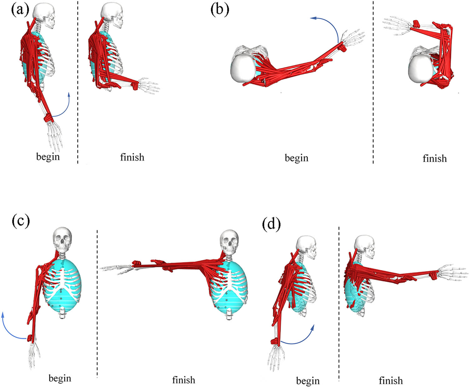
Figure 1
Simulation analysis of movement process: (a) elbow flexion, (b) horizontal adduction/abduction, (c) vertical abduction/adduction, and (d) flexion/extension.
This study uses joint movement angles as input data for upper limb muscle force simulation, can directly use the upper limb data included in the DAS3 model for simulation analysis. Simulation workflow consisted of three primary stages. First, the time–series joint angle data obtained from clinical measurements (Table 2) are converted into a .trc format file available in openSim and input it into the Inverse kinematics (IK) tool to generate motion data files (.mot) for the selected movements, with the processed IK data for the shoulder and elbow joints summarized (Tables 4 and 5), respectively. Subsequently, the Inverse dynamics analyzer was applied to compute the required joint moments. Finally, using a static optimization (SO) solver, the dynamic changes in muscle strength of the upper arm and forearm muscle groups throughout the entire rehabilitation cycle are calculated, and the biomechanical potential of the upper arm muscle groups being stretched and involved are analyzed. It should be noted that using static optimization for muscle force estimation does not necessarily mean that muscles will actively contribute during passive rehabilitation. This article uses hypothetical active motion simulation to select the action that stimulates the upper limb muscle group the most as the target trajectory for passive rehabilitation training.
2.3. Design of the upper limb rehabilitation mechanisms
Based on the physiological trajectories derived from the OpenSim simulations, two distinct types of upper limb rehabilitation mechanisms – an exoskeleton type and an end–effector type – were designed. Prior to structural modeling, the required DOF for each mechanism was calculated using the general mobility formula:
where F represents the total DOF of the mechanism, n denotes the number of moving links, P L is the number of lower kinematic pairs, and P H indicates the number of higher kinematic pairs.2.3.1. Exoskeleton mechanism design
According to the DOF analysis, the exoskeleton mechanism as a whole has five passive adjustable DOFs, but the active drive module is simplified to two core joint DOFs for analysis. Designed to fully enclose the upper limb and replicate natural human joint kinematics, the mechanism utilizes the upper and forearm parts of the model as driving linkages. The structural configuration comprises three serially connected modules: the shoulder, elbow, and wrist mechanisms (Figure 2).
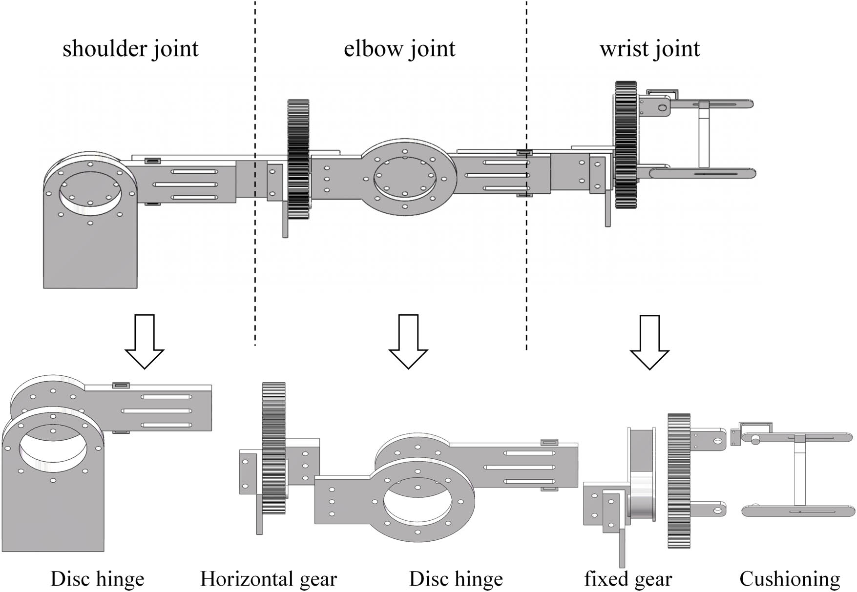
Figure 2
Exoskeleton mechanism.
The shoulder module features a 2–DOF design facilitating for horizontal adduction/abduction and flexion/extension via disc hinge connections. The elbow module provides a single–DOF motion for horizontal adduction/abduction, ensuring alignment between the mechanical hinges and the anatomical rotation axes. Adjustable link lengths and strap systems were incorporated to accommodate diverse anthropometric dimensions and minimize the misalignment–induced stress.
2.3.2. End–effector mechanism design
Conversely, the end–effector mechanism was conceptualized as a 3–DOF linkage system containing two lower pairs and two higher pairs. Unlike the exoskeleton, this mechanism operates in series with the biological limb, applying traction forces to the distal end (hand/wrist) to drive the proximal joints.
The system is composed of a multi–segment serial robotic arm, a traction device, and a terminal effector (Figure 3). The robotic arm utilizes revolute joints to achieve the necessary horizontal and oblique spatial displacements required for horizontal adduction/abduction and flexion/extension exercises. The terminal effector features a customized glove–type interface that secures the hand and transmits directional pulling forces via cables or steel bands, without directly constraining the intermediate elbow or shoulder joints.
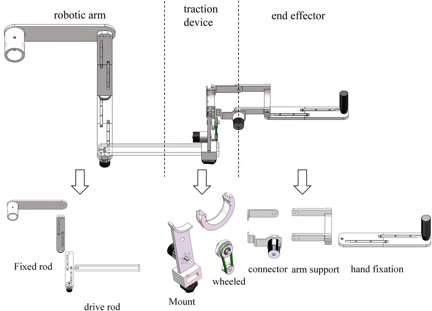
Figure 3
End–effector mechanism.
2.4. Co–simulation and performance evaluation protocol
To comparatively evaluate the trajectory adaptability and biomechanical safety of the two designed mechanisms, virtual prototype co–simulations and R 2 calculation were conducted. Before using ADAMS for simulation analysis, the two mechanism models were imported into the software for parameter settings. The link length was set to static, the model to aluminum alloy material in the software, and the fixed and rotating pairs were added.
2.4.1. Trajectory similarity analysis
The 3D models of both mechanisms were imported into ADAMS 2020 software, adjusting the model coordinate system. To ensure cross platform consistency, all models are defined in a unified global coordinate system (right–handed Cartesian system, with the origin at the shoulder joint center). Using the IK data generated in OpenSim (Tables 4 and 5) as a reference, the rotational pairs and mechanism drives of the two mechanisms are input in ADAMS to simulate the continuous motion of rehabilitation tasks. The center point of the mechanism end is set as the trajectory sampling point to obtain the motion trajectory of the mechanism. The spatial coordinates of the end–effectors were extracted from ADAMS and imported into MATLAB R2022b. To quantify the kinematic fidelity of the devices, the discrete Fréchet distance algorithm was employed to calculate the geometric similarity between the device–generated trajectories and the ideal human physiological trajectories. A smaller Fréchet distance indicates higher trajectory precision.
2.4.2. Analysis of trajectory determination coefficient
To quantitatively evaluate the trajectory tracking performance of different rehabilitation mechanisms, the similarity between the mechanism trajectory and human model trajectory was evaluated through the coefficient of determination (R 2). The trajectory data of the human body model and the trajectory data of the two mechanisms were sampled and aligned in a unified coordinate system according to time (Tables 6 and 7) and the R 2 of the trajectories of the two mechanisms was calculated. The formula for R 2 calculation is as follows:
where R 2 represents the coefficient of determination of the mechanism, y i is the trajectory value of the human body model, ŷ is the trajectory value of the mechanism, and ȳ is the mean trajectory value of the human body model.Table 6
Horizontal adduction/abduction trajectory data
| Time | Human X | Human Y | Exo X | Exo Y | End X | End Y |
|---|---|---|---|---|---|---|
| 0 | 0.5500 | 0.0000 | 0.5497 | 0.0174 | 0.5470 | −0.0519 |
| 0.25 | 0.5499 | 0.0088 | 0.5493 | 0.0267 | 0.5487 | −0.0335 |
| 0.5 | 0.5488 | 0.0348 | 0.5479 | 0.0459 | 0.5499 | 0.0073 |
| 0.75 | 0.5439 | 0.0771 | 0.5438 | 0.0778 | 0.5459 | 0.0650 |
| 1 | 0.5315 | 0.1335 | 0.5343 | 0.1231 | 0.5338 | 0.1267 |
| 1.25 | 0.5070 | 0.2006 | 0.5133 | 0.1861 | 0.5112 | 0.1928 |
| 1.5 | 0.4669 | 0.2728 | 0.4739 | 0.2620 | 0.4785 | 0.2564 |
| 1.75 | 0.4089 | 0.3431 | 0.4099 | 0.3422 | 0.4324 | 0.3197 |
| 2 | 0.3341 | 0.4042 | 0.3229 | 0.4113 | 0.3639 | 0.3848 |
| 2.25 | 0.2462 | 0.4492 | 0.2220 | 0.4578 | 0.2684 | 0.4421 |
| 2.5 | 0.1516 | 0.4740 | 0.1184 | 0.4777 | 0.1482 | 0.4769 |
| 2.75 | 0.0580 | 0.4776 | 0.0240 | 0.4739 | 0.0212 | 0.4763 |
| 3 | −0.0275 | 0.4625 | −0.0528 | 0.4544 | −0.0844 | 0.4450 |
| 3.25 | −0.0999 | 0.4337 | −0.1105 | 0.4280 | −0.1563 | 0.4026 |
| 3.5 | −0.1569 | 0.3975 | −0.1546 | 0.3992 | −0.1974 | 0.3668 |
| 3.75 | −0.1984 | 0.3602 | −0.1905 | 0.3682 | −0.2185 | 0.3434 |
| 4 | −0.2265 | 0.3268 | −0.2183 | 0.3373 | −0.2321 | 0.3256 |
| 4.25 | −0.2439 | 0.3008 | −0.2373 | 0.3111 | −0.2404 | 0.3133 |
| 4.5 | −0.2531 | 0.2845 | −0.2484 | 0.2930 | −0.2435 | 0.3085 |
| 4.75 | −0.2559 | 0.2790 | −0.2527 | 0.2851 | −0.2409 | 0.3124 |
| 5 | −0.2600 | 0.2751 | −0.2517 | 0.2844 | −0.2379 | 0.3129 |
Table 7
Flexion/extension trajectory data
| Time | Human X | Human Y | Exo X | Exo Y | End X | End Y |
|---|---|---|---|---|---|---|
| 0 | −0.2800 | −0.4734 | −0.2648 | −0.4820 | −0.3173 | −0.4490 |
| 0.25 | −0.2732 | −0.4773 | −0.2574 | −0.4860 | −0.3027 | −0.4590 |
| 0.5 | −0.2527 | −0.4885 | −0.2428 | −0.4935 | −0.2703 | −0.4789 |
| 0.75 | −0.2183 | −0.5048 | −0.2176 | −0.5051 | −0.2226 | −0.5029 |
| 1 | −0.1698 | −0.5231 | −0.1801 | −0.5197 | −0.1696 | −0.5232 |
| 1.25 | −0.1076 | −0.5394 | −0.1232 | −0.5360 | −0.1090 | −0.5391 |
| 1.5 | −0.0334 | −0.5490 | −0.0465 | −0.5480 | −0.0462 | −0.5480 |
| 1.75 | 0.0499 | −0.5477 | 0.0485 | −0.5479 | 0.0235 | −0.5494 |
| 2 | 0.1382 | −0.5323 | 0.1517 | −0.5287 | 0.1096 | −0.5389 |
| 2.25 | 0.2264 | −0.5012 | 0.2512 | −0.4892 | 0.2107 | −0.5080 |
| 2.5 | 0.3091 | −0.4549 | 0.3388 | −0.4330 | 0.3189 | −0.4481 |
| 2.75 | 0.3817 | −0.3960 | 0.4087 | −0.3678 | 0.4157 | −0.3597 |
| 3 | 0.4409 | −0.3288 | 0.4589 | −0.3031 | 0.4827 | −0.2623 |
| 3.25 | 0.4856 | −0.2583 | 0.4922 | −0.2453 | 0.5196 | −0.1777 |
| 3.5 | 0.5161 | −0.1900 | 0.5149 | −0.1933 | 0.5363 | −0.1195 |
| 3.75 | 0.5348 | −0.1286 | 0.5311 | −0.1428 | 0.5429 | −0.0866 |
| 4 | 0.5445 | −0.0776 | 0.5417 | −0.0953 | 0.5463 | −0.0633 |
| 4.25 | 0.5486 | −0.0397 | 0.5471 | −0.0564 | 0.5479 | −0.0479 |
| 4.5 | 0.5498 | −0.0165 | 0.5492 | −0.0300 | 0.5483 | −0.0428 |
| 4.75 | 0.5499 | −0.0086 | 0.5497 | −0.0184 | 0.5475 | −0.0501 |
| 5 | 0.5501 | −0.0089 | 0.5504 | −0.0094 | 0.5575 | −0.0511 |
2.4.3. Joint torque evaluation
To assess the biomechanical safety, ADAMS dynamic simulation was used to monitor the rotational torque on the shoulder, elbow, and wrist joints of two mechanisms during the execution of selected rehabilitation exercises. Excessive joint torque concentrations at specific anatomical nodes were established as the primary indicator of potential secondary injury risk during passive training. According to clinical studies on the risk of shoulder subluxation in stroke patients with soft paralysis [18,19], the maximum safe range of joint torque for rehabilitation training is 30–50% of the average maximum isometric contraction torque of adult upper limb joints. In this study, the median value of 40 Nm was taken as the preliminary safety threshold for joint torque in upper limb rehabilitation training.
3. Results
3.1. Kinematic analysis and selection of rehabilitation movements
Initial kinematic measurements of the six fundamental passive upper limb rehabilitation movements are summarized in Table 2. Analysis of the average ROM across five trials revealed that the rotational amplitudes for shoulder internal/external rotation and elbow internal/external rotation were small. Consequently, these two movements were excluded from further biomechanical evaluation.
The remaining four movements (elbow flexion, horizontal adduction/abduction, vertical abduction/adduction, flexion/extension) were simulated in OpenSim to analyze dynamic muscle force variations. As illustrated in Figure 4, the forearm (red lines) and upper arm (black lines) muscle groups exhibited distinct activation patterns across the different exercises.
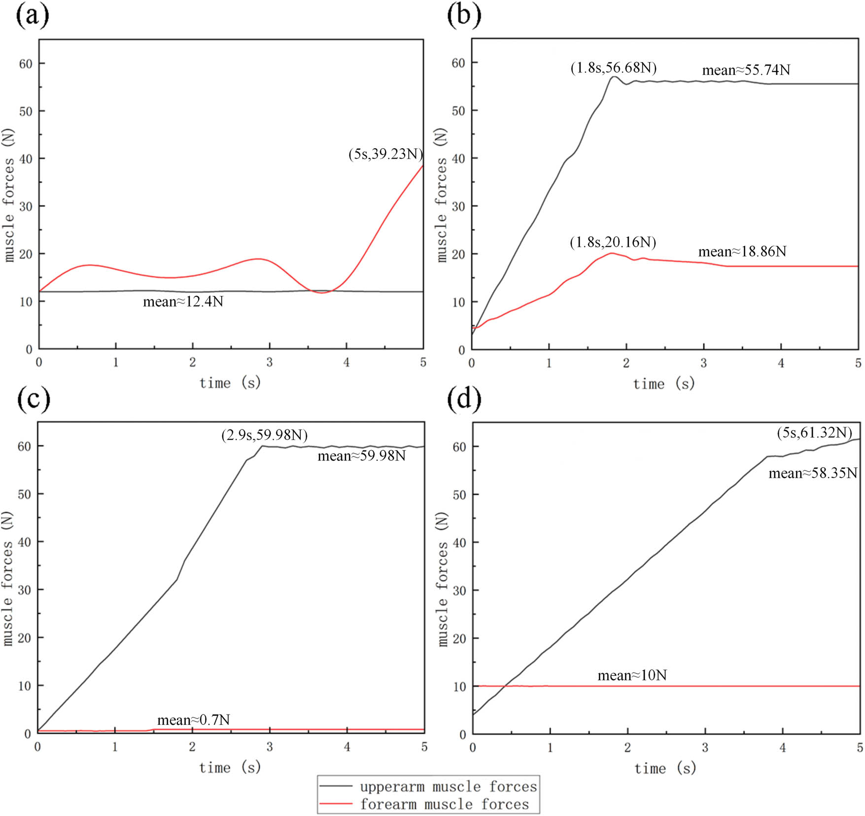
Figure 4
Changes in upper limb muscle force: (a) elbow flexion, (b) horizontal adduction/abduction, (c) vertical abduction/adduction, and (d) flexion/extension.
During elbow flexion (Figure 4a), the forearm muscle force showed significant variation, peaking at 39.23 N (at 5 s, with a flexion angle of 91.5°), while the upper arm force remained relatively stable at approximately 12.4 N. In horizontal adduction/abduction (Figure 4b), both forearm and upper arm muscles exhibited notable synchronous engagement, peaking at 20.16 N (28.9°) and 56.68 N (36.8°), and stabilizing around 18.86 N and 55.74 N during the maintenance phase, respectively. In vertical abduction/adduction (Figure 4c), upper arm force peaked sharply at 59.98 N, but forearm activation was negligible (0.7 N). In flexion/extension (Figure 4d), the upper arm muscle force varied significantly, reaching a peak of 61.32 N (89.1°); conversely the forearm force remained constant near 10 N.
Muscle force data sampling was performed on the movement process of four actions, and the actions with high muscle force activation were screened through RMS analysis. The formula for calculating RMS is as follows:
Collectively, based on the muscle force data calculated by the formula (Table 8), the involvement of the upper arm is relatively high in horizontal adduction/abduction, vertical abduction/adduction, and flexion/extension. Elbow flexion shows significant forearm activation but incomplete upper arm training. To ensure full participation and structural verification of the upper limbs, horizontal adduction/abduction and flexion/extension were selected as the target guidance trajectories for the mechanism simulation. The selected action space trajectory generated through OpenSim is shown in Figure 5.Table 8
Muscle strength RMS data
| Time (s) | Elbow flexion | Horizontal adduction/abduction | Vertical abduction/adduction | Flexion/extension | ||||
|---|---|---|---|---|---|---|---|---|
| Upper (N) | Fount (N) | Upper (N) | Fount (N) | Upper (N) | Fount (N) | Upper (N) | Fount (N) | |
| 0 | 12.40 | 12.40 | 4.26 | 4.13 | 6.00 | 0.49 | 7.00 | 10.00 |
| 0.25 | 12.45 | 13.50 | 11.18 | 6.27 | 6.00 | 0.65 | 7.00 | 10.05 |
| 0.5 | 12.35 | 16.80 | 18.10 | 8.41 | 8.50 | 0.75 | 9.50 | 9.95 |
| 0.75 | 12.48 | 16.70 | 25.02 | 10.55 | 12.50 | 0.68 | 13.20 | 10.08 |
| 1 | 12.32 | 15.70 | 31.94 | 12.69 | 17.50 | 0.72 | 18.50 | 9.92 |
| 1.25 | 12.43 | 15.11 | 38.86 | 14.83 | 18.50 | 0.63 | 19.20 | 10.03 |
| 1.5 | 12.37 | 14.50 | 45.78 | 16.97 | 27.40 | 0.75 | 28.50 | 9.97 |
| 1.75 | 12.41 | 13.40 | 55.20 | 19.80 | 28.50 | 0.69 | 29.80 | 10.01 |
| 2 | 12.39 | 14.41 | 55.74 | 18.80 | 37.50 | 0.71 | 39.80 | 9.99 |
| 2.25 | 12.46 | 16.19 | 55.76 | 18.61 | 39.20 | 0.66 | 41.50 | 10.06 |
| 2.5 | 12.34 | 18.53 | 55.73 | 18.34 | 47.80 | 0.74 | 50.80 | 9.94 |
| 2.75 | 12.44 | 20.21 | 55.74 | 18.20 | 53.10 | 0.67 | 52.60 | 10.02 |
| 3 | 12.36 | 18.50 | 55.75 | 18.20 | 59.40 | 0.73 | 54.40 | 9.98 |
| 3.25 | 12.42 | 16.80 | 55.77 | 18.17 | 59.30 | 0.64 | 56.20 | 10.04 |
| 3.5 | 12.38 | 15.10 | 55.74 | 18.15 | 59.50 | 0.76 | 58.00 | 9.96 |
| 3.75 | 12.40 | 12.60 | 55.73 | 18.14 | 59.60 | 0.70 | 58.40 | 10.07 |
| 4 | 12.41 | 15.80 | 55.52 | 18.11 | 59.70 | 0.70 | 59.60 | 9.93 |
| 4.25 | 12.39 | 19.82 | 55.71 | 18.09 | 59.80 | 0.68 | 59.70 | 10.00 |
| 4.5 | 12.40 | 27.35 | 55.78 | 18.04 | 59.80 | 0.72 | 60.20 | 10.00 |
| 4.75 | 12.40 | 34.18 | 55.76 | 18.01 | 59.70 | 0.69 | 61.50 | 10.00 |
| 5 | 12.40 | 39.23 | 55.72 | 18.01 | 59.70 | 0.71 | 62.40 | 10.00 |
| RMS | 12.401 | 19.200 | 45.997 | 15.848 | 42.840 | 0.691 | 42.727 | 10.010 |
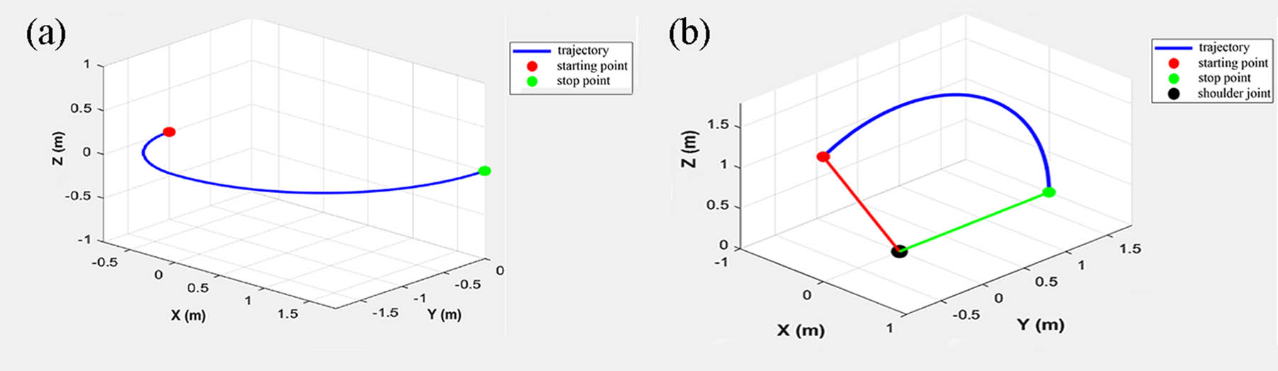
Figure 5
Upper limb model motion trajectory: (a) Horizontal Adduction/abduction trajectory and (b) flexion/extension trajectory.
3.2. Motion trajectory simulation and similarity analysis
Based on the mechanism design principles (exoskeleton confirmed as 2–DOF and end–effector as 3–DOF linkage systems, as detailed in Table 9), the virtual prototypes were driven in ADAMS. Both mechanisms successfully completed the assigned rehabilitation motions without kinematic singularities (Figure 6).
Table 9
Number of mechanism components
| Mechanism type | Movable links in mechanism (n) | Lower pairs (PL) | Higher pairs (PH) | DOF (F) |
|---|---|---|---|---|
| Exoskeleton | 2 | 2 | 0 | 2 |
| End–effector | 3 | 2 | 2 | 2 |
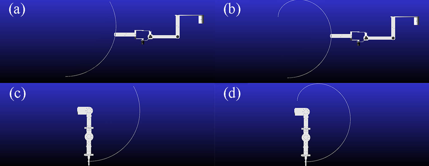
Figure 6
End of mechanism trajectories: (a) end–effector during flexion/extension, (b) end–effector trajectory during adduction/abduction, (c) exoskeleton–type during flexion/extension, and (d) exoskeleton during horizontal adduction/abduction.
The kinematic fidelity of the mechanisms was quantified using discrete Fréchet distance analysis in MATLAB, comparing the device–generated trajectories with the natural physiological trajectories (Figure 7).
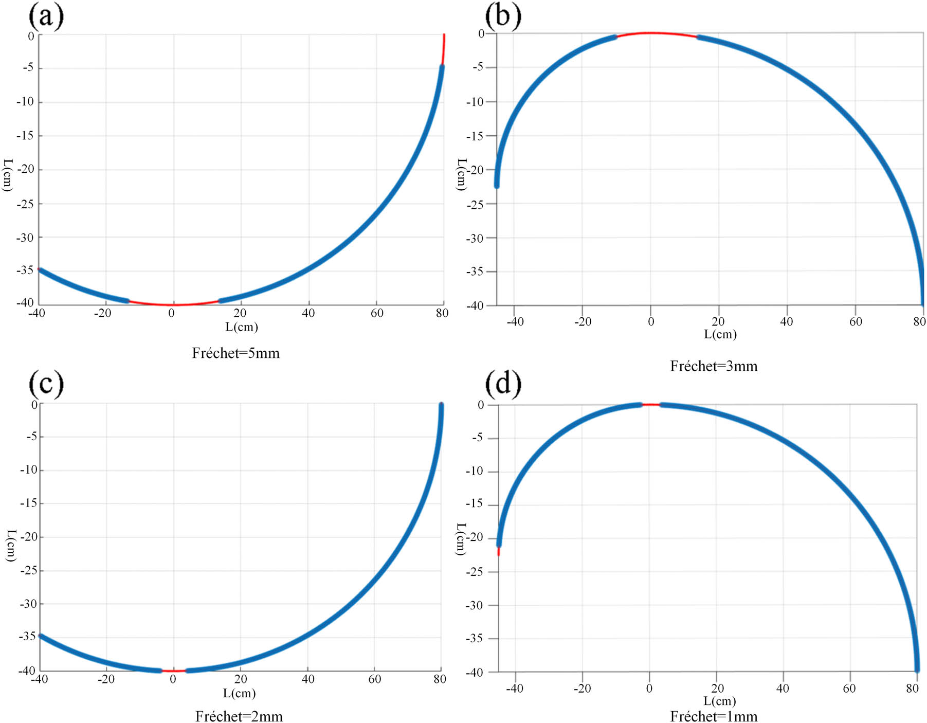
Figure 7
Trajectory fitting: (a) end–effector during flexion/extension, (b) end–effector during horizontal adduction/abduction, (c) exoskeleton during flexion/extension, and (d) exoskeleton during horizontal adduction/abduction.
The simulation results demonstrated a significant discrepancy in trajectory precision between the two device types. For the end–effector mechanism, the Fréchet distance was calculated as 5 mm during flexion/extension (Figure 7a) and 3 mm during horizontal adduction/abduction (Figure 7b). In contrast, for the exoskeleton mechanism, the Fréchet distance was calculated as 2 mm during flexion/extension (Figure 7c) and 1 mm during horizontal adduction/abduction (Figure 7d). The data indicate that the exoskeleton–type device achieves extremely high similarity to natural human motion (errors controlled within ≤2 mm) due to independent joint alignment, whereas the end–effector device exhibits a comparatively weaker fit (errors controlled within ≤5 mm).
3.3. Calculation and analysis of trajectory determination coefficient
R 2 was used to quantify the similarity between the trajectory of the mechanism and the reference human motion trajectory. R 2 value close to 1 indicates a higher degree of trajectory matching. The trajectory data (Tables 6 and 7) were substituted in the determination coefficient formula (Equation (2)) for calculation.
According to the formula, the R 2 values of the end–effector mechanism in two movements are 0.9942 and 0.9910, while the R 2 values of the exoskeleton mechanism in two movements are 0.9988 and 0.9975, respectively. The overall trajectory difference is shown in Figure 8.
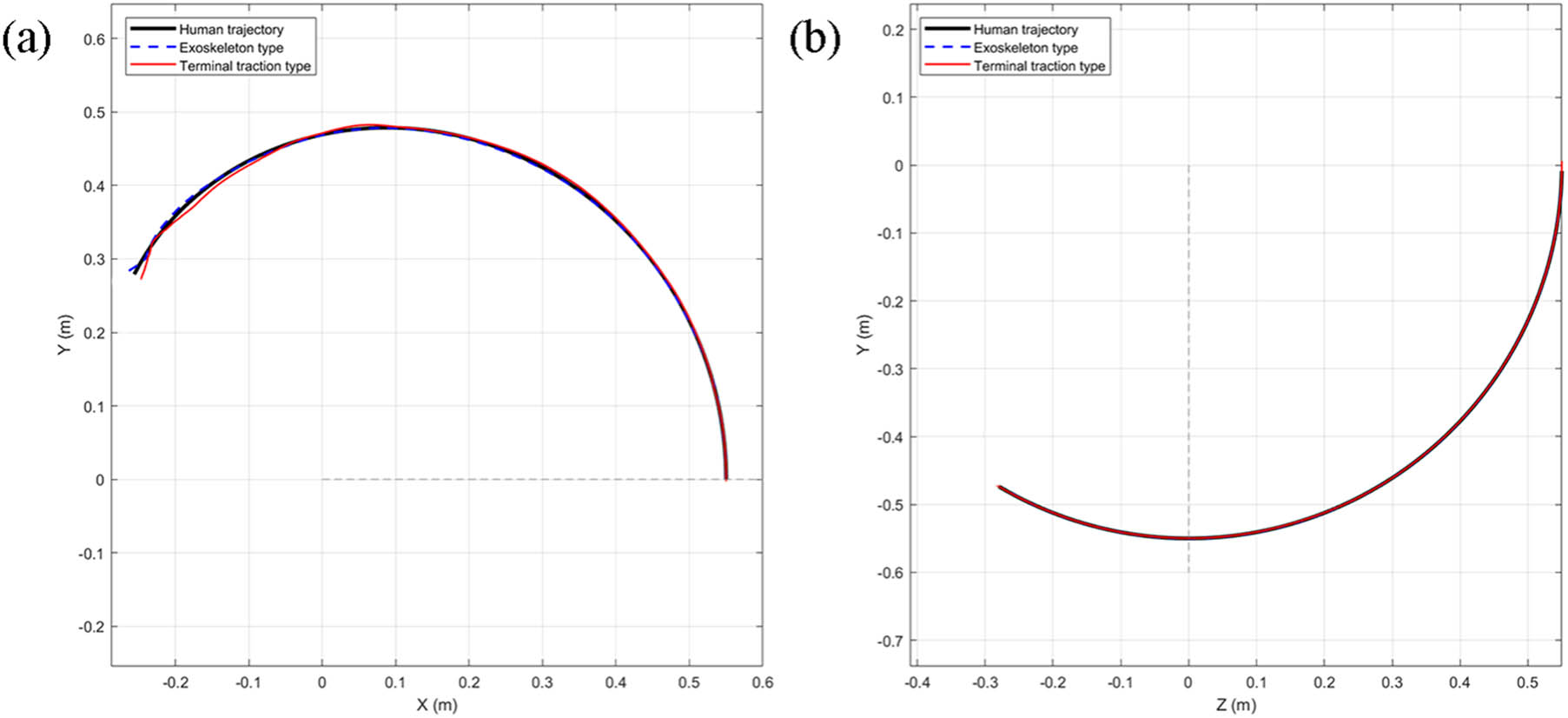
Figure 8
Comparison of R 2 data trajectories at the end of mechanisms: (a) horizontal adduction/abduction comparison and (b) flexion/extension comparison.
3.4. Joint torque evaluation and biomechanical safety
The dynamic rotational torques experienced by the upper limb joints during the execution of the rehabilitation trajectories are presented in Figure 9.
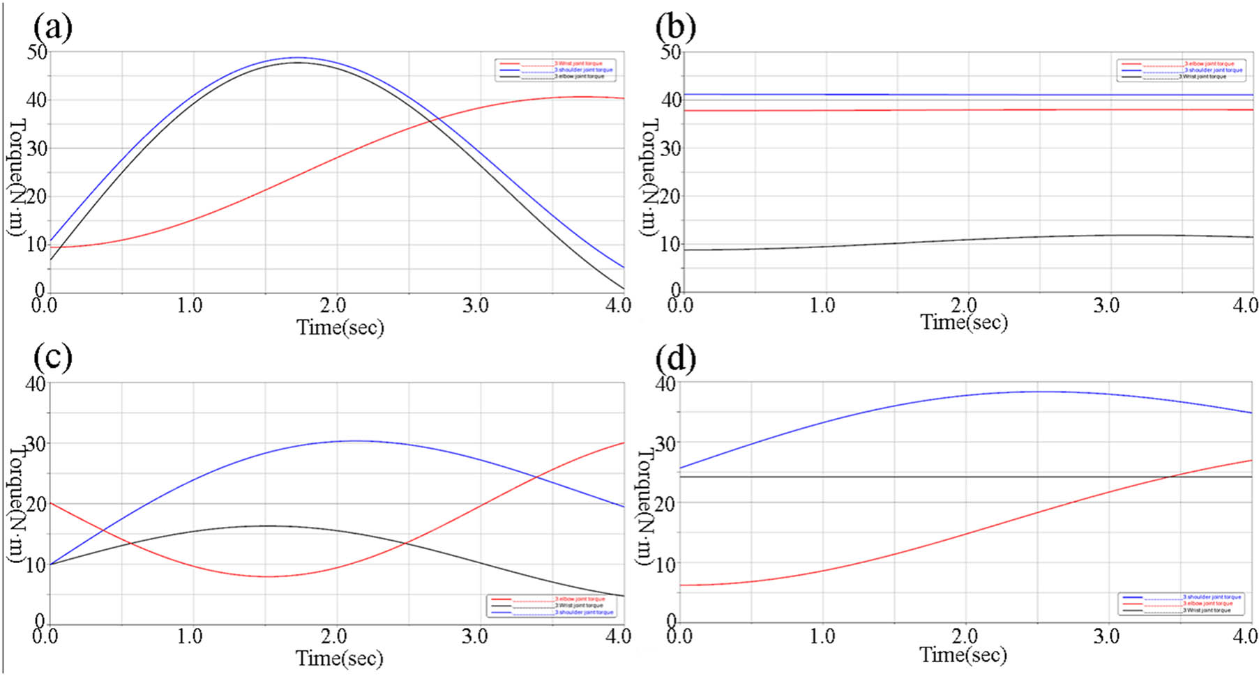
Figure 9
Variation in joint torque: (a) flexion/extension with end–effector mechanism, (b) horizontal adduction/abduction with end–effector mechanism, (c) flexion/extension with exoskeleton mechanisms, and (d) horizontal adduction/abduction with exoskeleton mechanisms.
During both flexion/extension and horizontal adduction/abduction, simulation results for the end–effector mechanism (Figure 9a and b) revealed significant stress concentrations at the distal joints, the joint moments for the wrist and elbow exhibited sharp fluctuations, > 40 Nm at their peaks. Although the overall moment changes were relatively modest during horizontal movements, the wrist joint torque was still > 40 Nm, and the shoulder joint approached this limit.
Conversely, the exoskeleton mechanism demonstrated a highly balanced torque distribution (Figure 9c and d). During flexion/extension, all joint torque variations remained strictly <40 Nm. Similarly, throughout the entire movement cycle of horizontal adduction/abduction, the joint moment fluctuations for the shoulder, elbow, and wrist stayed consistently <30 Nm. These findings quantitatively confirm that the exoskeleton design significantly reduces abnormal joint loading compared to the end–effector approach.
4. Discussion
The primary objective of this study was to compare the kinematic trajectory adaptability and biomechanical safety (joint torque variations) of two mainstream upper limb rehabilitation mechanisms – exoskeleton and end–effector types – during passive training. By integrating musculoskeletal modeling with dynamic mechanical simulation, we quantitatively evaluated both devices under identical physiological movement conditions.
4.1. Kinematic fidelity and structural mechanisms
Our trajectory similarity analysis utilizing the discrete Fréchet distance revealed that the exoskeleton mechanism significantly outperformed the end–effector mechanism (errors ≤2 mm vs ≤5 mm). This discrepancy fundamentally stems from their structural paradigms. The exoskeleton is designed with joint axis alignment, meaning its mechanical hinges physically coincide with the patient’s anatomical rotation centers. This configuration allows for precise, independent control of individual joint angles, effectively replicating complex three–dimensional human motions.
Conversely, the end–effector mechanism operates by constraining only the distal extremity (the hand or wrist) and relies on IK to drive the entire upper limb. Because it lacks direct control over the intermediate joints (elbow and shoulder), spatial deviations are inevitable when simulating multi–joint coordinated movements, leading to a lower fit to natural physiological patterns.
In coefficient of determination analysis, exoskeleton–type trajectory (R 2 ≥ 0.9975) was better than end–effector–type trajectory (R 2 ≥ 0.9910), proving that exoskeleton mechanisms are superior to end effector mechanisms in trajectory fitting.
4.2. Biomechanical safety and clinical implications
A critical finding of this study is the drastic difference in joint torque distribution between the two mechanisms. During passive rehabilitation exercises, the end–effector device generated excessive torques (>40 Nm) at the wrist and elbow joints. From a biomechanical perspective, applying a driving force at the terminal end creates a significant lever–arm effect. To overcome the inertia and gravity of the entire arm, the distal actuator must exert substantial force, which translates into concentrated stress at the proximal joints.
For patients in the early flaccid stage of stroke recovery (Brunnstrom Stage I), muscle tone is virtually absent, and the ligaments are highly vulnerable. Subjecting these patients to concentrated torques > 40 Nm poses a severe risk of secondary injuries, such as shoulder subluxation or ligament sprains. Therefore, our results strongly suggest that end–effector systems require highly advanced force–compliance algorithms (e.g., impedance/admittance control) to mitigate biomechanical risks, as traditional rigid position control is unsafe for early–stage passive training.
In contrast, the exoskeleton mechanism maintained balanced joint moments strictly between 30 and 40 Nm throughout all movement cycles. By applying distributed forces locally at each corresponding joint, the exoskeleton eliminates the long lever–arm effect. This makes the exoskeleton intrinsically safer and highly suitable for passive motion assistance and ROM recovery in early–stage stroke rehabilitation. However, it is worth noting that while exoskeletons offer superior joint protection, they demand precise donning procedures; any misalignment between the mechanical and anatomical axes during practical application could introduce parasitic forces, necessitating adjustable and compliant coupling designs.
4.3. Limitations and future work
Despite the comprehensive framework proposed in this study, several limitations should be acknowledged.
Trajectory similarity does not necessarily reflect actual limb motion during human–robot interaction, as relative displacement may occur due to soft tissue deformation, compliance, and alignment errors, potentially leading to overestimated performance. The current model does not fully represent the complexity of the shoulder complex. The dynamic motion of the shoulder joint center and simplified modeling assumptions may introduce kinematic incompatibility and increased interaction forces. Human–robot interface mismatch remains a challenge. Although adjustable mechanisms are included, precise alignment is difficult to achieve due to anatomical variability, resulting in unavoidable trade–offs that were not fully quantified.
Results are based on simulations without experimental validation. Key real–world factors, such as actuator dynamics, control delays, and user adaptation, were not considered, limiting clinical applicability.
Future work will address these limitations by developing subject–specific and compliant human–robot interaction models, incorporating detailed shoulder complex kinematics, and improving interface design for better alignment and adaptability. Moreover, physical prototypes will be constructed and validated through experimental studies involving both healthy participants and stroke patients, using techniques such as motion capture, surface electromyography, and force/torque sensing. These efforts will enable a more realistic assessment of device performance and support the translation of simulation findings into clinical applications.
5. Conclusion
This study systematically compared the kinematic trajectory adaptability and biomechanical safety of exoskeleton–type and end–effector–type upper limb rehabilitation mechanisms through musculoskeletal and dynamic co–simulations. Initial biomechanical analysis using OpenSim identified horizontal adduction–abduction and anterior–posterior flexion as the most effective passive exercises for comprehensive upper limb muscle engagement during the flaccid stage of stroke recovery, establishing them as optimal guiding trajectories for subsequent mechanism design.
Comparative simulations demonstrated that the exoskeleton mechanism achieves significantly higher fidelity in replicating natural human arm trajectories, with discrete Fréchet distance errors ≤2 mm. In contrast, the end–effector system exhibited a lower fit to physiological movement patterns, showing tracking errors ≤5 mm. In coefficient of determination analysis, exoskeleton–type trajectory with R 2 ≥ 0.9975 was better than end–effector–type trajectory with R 2 ≥ 0.9910. Furthermore, dynamic joint torque evaluations revealed that the exoskeleton device effectively maintains balanced rotational moments across the shoulder, elbow, and wrist joints, keeping them well below 40 Nm. Conversely, the end–effector design generates concentrated lever–arm forces that result in excessive torques at the distal joints, posing potential stress injury risks during passive training.
Ultimately, exoskeleton–type mechanisms exhibit clear advantages in both trajectory precision and joint protection, making them highly suitable for passive motion assistance and ROM recovery in early–stage rehabilitation. While end–effector systems offer structural simplicity and spatial flexibility for complex motions, their safe application necessitates the integration of advanced force–compliance algorithms to mitigate concentrated terminal forces and ensure biomechanical safety.
Funding information
This research did not receive any specific grant from funding agencies in the public, commercial, or not-for-profit sectors.
Author contributions
Haoyu Han: Writing – original draft, Li Feng: Writing – review and editing, and Qinghui Zhu: Software.
Conflict of interest statement
The authors declare that they have no known competing financial interests or personal relationships that could have appeared to influence the work reported in this manuscript. The authors confirm that this manuscript has not been published previously and is not currently under consideration for publication elsewhere.
Data availability statement
The datasets supporting this study are available from the corresponding author upon reasonable request.