
1. Introduction
Musculoskeletal system (MSKS) modelling methods are increasingly used in biomechanical analysis to estimate muscle and joint reaction forces during human movement. This approach has been applied to both static postures [1,2] and dynamic activities, for both healthy individuals and those with MSKS disorders [3–9]. Such analyses are performed using several software platforms and a variety of MSKS models.
A standard MSKS model developed in particular software is typically based on a limited number of cadaver datasets. As a result, these models may differ from each other and fail to reflect individual anatomical variability, such as geometry of bone segments, location of muscle attachment points, or muscle structural parameters [10–12]. In addition, various models of particular joints, in terms of the number of degrees of freedom (DOF) and definition of local coordinate systems, affect MSKS kinematics [5,13]. This raises the question of how differences in the model structure influence the calculated parameters (value, direction) of the MSKS loadings.
As the number of studies based on MSKS modelling increases, the reliability of the results obtained from different systems is becoming increasingly important. The variety of existing MSKS models implemented in different modelling environments can lead to significant differences in the obtained results, such as joint angles [11,13,14], joint torques [11,14], muscle moment arms [14], estimated muscle forces [14] and joint reaction forces [12,15]. Previous studies (e.g. [5,11,12,14–21]) have reported discrepancies in biomechanical results obtained using MSKS modelling systems. These differences have been observed in comparisons between different modelling systems (e.g. OpenSim, AnyBody, MATLAB) [14–17,21], musculoskeletal models [11,12] or modelling approaches [5,18–20]. Direct comparisons between different modelling environments reveal discrepancies in the estimated values and directions of the muscle forces as well as moments and reactions acting in the joints of the lower limb. The diversity of the results obtained from different software may occur due to several reasons, including the geometry of the MSKS model, the applied scaling laws, or the parameters used in the optimisation procedure. In AnyBody, bone segments are first scaled in the longitudinal direction and then scaled in width to obtain a specified mass (dynamic trial). Several scaling approaches can be used for this purpose, for example, the length–mass or length–mass–fat scaling law [22]. In contrast, in OpenSim, segments are scaled in the principal axis direction to fit the position of the joint centres and in the perpendicular direction to fit pairs of landmarks (static trial) [23]. The static optimisation method used for estimating muscle forces in OpenSim most commonly minimises the sum of muscle activations [23]. In AnyBody, static optimisation is most commonly used to minimise the polynomial muscle recruitment criterion [15,22].
Earlier studies confirm that these factors significantly impact sagittal ankle and hip angles, knee moments and the muscle force magnitudes of the triceps surae group and the biceps femoris short head [14]. Differences in the forces of these muscles are assumed to be due to differences in basic anthropometric and anatomical parameters (mass, length and inertial parameters of the segments, muscle properties, muscle moment arms). Changes in the segment scaling procedure have been shown to affect joint kinematics [5] and kinetics, as well as muscle and joint reaction forces [24]. Optimisation methods also influence hip joint reaction forces and muscle activation patterns [16,20,25]. Wagner et al. [21] showed substantial differences between models (AnyBody, OpenSim, MATLAB), taking into account the quadriceps moment arms, distributions in quadriceps muscle recruitment and tibio-femoral joint reaction forces. Increases in some muscle forces were associated with decreases in muscle moment arms to obtain the same resultant moment [26].
It should be noted that models available in software packages are continuously updated, and changes are largely focused on the lower extremity. For example, the authors of the AnyBody Modeling System originally developed TLEM 1.1 (Twente Lower Extremity Model) consisting of the lower limb and pelvis [27], which was updated to TLEM 2.0 [28]. The update of the AnyBody model aimed to incorporate more anatomically accurate geometries of the lower limb bone segments and to improve muscle path definitions. In addition, TLEM 2.0 was specifically developed to facilitate integration with imaging-based scaling techniques. It is important to note that previously mentioned research often employed different modelling environments when assessing the influence of various models on simulation results. In such cases, the observed differences could be affected simultaneously by multiple factors: not only the geometry of the MSKS model itself, but also the number of unlocked degrees of freedom for particular joints, scaling methods, optimisation criteria, or computational algorithms implemented in the respective software. This heterogeneity of modelling methodologies makes it difficult to fully understand the problem.
To the authors’ knowledge, no previous study has directly compared TLEM 1.1 and TLEM 2.0 within the AnyBody Modeling System while applying identical scaling laws and optimisation procedures. The aim of this study was to assess whether structural differences between MSKS models TLEM 1.1 and TLEM 2.0, implemented in the same modelling environment (AnyBody Modeling System) and analysed using identical scaling laws and optimisation procedures, lead to differences in predicted muscle forces and joint reaction forces (hip, knee and ankle) during gait. The research questions focused on whether TLEM 1.1 and TLEM 2.0 generate significantly different time waveforms of active muscle forces and whether the models differ in their predicted joint reaction force components. It was hypothesised that structural differences between TLEM 1.1 and TLEM 2.0, including modification of pelvis and femur geometry, inclusion of the fibula, and updated muscle attachment points and pathways [10,27–29], would significantly influence the results.
2. Materials and methods
A detailed comparison of two musculoskeletal models available in the AnyBody Modeling System (version 7.3, AnyBody Technology A/S, Aalborg, Denmark) repository (TLEM 1.1/TLEM 2.0) is provided in Tables 1 and 2.
Table 1
Comparison between TLEM 1.1 and TLEM 2.0 models implemented in the AnyBody Modeling System repository
| TLEM 1.1 | TLEM 2.0 | |||
|---|---|---|---|---|
| Information included in the literature [27–29] | ||||
| Cadaver | Men, 77 years, 1.74 m, body mass 105 kg | Men, 85 years, estimated mass of leg – 45 kg; leg length – 813 mm | ||
| Segments | Pelvis, right and left: femur, patella, tibia, talus, foot (consisting of hindfoot, midfoot, phalanges) | Pelvis, right and left: femur, patella, tibia (including fibula), talus, foot (consisting of hindfoot, midfoot, phalanges) | ||
| Joints and DOF | 21 DOF, 11 joints: L5S1, right and left: hip, knee, patellofemoral, talocrural, subtalar | |||
| Density parameters | x | Bone: 1,500 kg/m3; Muscle: 1,060 kg/m3; Fat: 900 kg/m3 | ||
| Inertial parameters | Segment mass and centre of mass were estimated using established anthropometric regression. Moments of inertia were calculated about the transversal and longitudinal axes of the segment | Segment mass, centre of mass, and also principal axes of inertia and moment of inertia were calculated for each segment, based on the segmented bone, muscle and fat volumes, using SolidWorks® 2013 | ||
| Muscle | 58 muscles divided into 163 branches per leg | 55 muscles divided into 166 branches per leg | ||
| Muscle parameters | The muscle–tendon architecture dataset (muscle fibre length, physiological cross-sectional area, the pennation angles and tendon length) was adapted from the original TLEM dataset [27] | |||
| Nominal fibre lengths and physiological cross-sectional area (PCSA) were adapted from the Klein-Horsman et al. [27] dataset | Fibre lengths were individually scaled, comparing the total length of the muscle-tendon elements in the TLEM 1.1 and in the TLEM 2.0 dataset | |||
| PCSA were calculated taking into account the scaled fibre lengths, the pennation angles and the measured muscle volumes | ||||
| Wrapping muscles | Illiacus, Psoas Major, Gastrocnemius | Illiacus, Psoas Major, Gluteus Maximus, Quadiceps Femoris, Hamstrings, Gastrocnemius | ||
| Parameters included in the AnyBody Modeling System for standard model | ||||
| Body parameters of standard model | Body mass = 75 kg | Body mass = 75 kg | ||
| Height = 1.80 m | Height = 1.75 m | |||
| Fat percent = (−0.09 + 0.0149 BMI − 0.00009 BMI2) × 100 | ||||
| Segment mass (kg) | Pelvis = 10.65 | Shank = 4.00 | Pelvis = 11.222 | Shank = 3.6287 |
| Patella = 0.00 | Talus = 0.26 | Thigh = 6.0191 | Talus = 0.2605 | |
| Thigh = 7.00 | Foot = 1.04 | Patella = 0.025 | Foot = 0.7226 | |
| Segments length, width (m) | PelvisWidth = 0.16 | KneeWidth = 0.0975 | PelvisWidth = 0.1686 | KneeWidth = 0.0975 |
| HeelHeight = 0.05 | AnkleWidth = 0.0753 | |||
Table 2
The completed list of the analysed muscle actuators available in the TLEM 1.1 and TLEM 2.0 models: number of muscle elements representing the muscle actuators, type of the path line
| Muscle | TLEM 1.1 | TLEM 2.0 | TLEM 1.1 | TLEM 2.0 | Muscle | TLEM 1.1 | TLEM 2.0 | TLEM 1.1 | TLEM 2.0 |
|---|---|---|---|---|---|---|---|---|---|
| S/WS/VP | #Elements | S/WS/VP | #Elements | ||||||
| Add. Brev. Distal | S | S | 2 | 2 | Obturator Ext. Sup. | VP | VP | 3 | 3 |
| Add. Brev. Mid | S | S | 2 | 2 | Obturator Int. | VP | VP | 3 | 6 |
| Add. Brev. Prox. | S | S | 2 | 2 | Pectineus | S | S | 4 | 4 |
| Add. Long. | S | S | 6 | 6 | Peroneus Brevis | VP | VP | 3 | 3 |
| Add. Mag. Distal | S | S | 3 | 3 | Peroneus Long. | VP | VP | 3 | 3 |
| Add. Mag. Mid | S | S | 6 | 6 | Peroneus tert. | VP | - | 3 | - |
| Add. Mag. Prox. | S | S | 4 | 4 | Piriformis | S | S | 1 | 1 |
| Biceps Fem. CB | S | WS | 3 | 3 | Plantaris | S | WS | 1 | 1 |
| Biceps Fem. CL | S | WS | 1 | 1 | Popliteus | VP | VP | 2 | 3 |
| Ext. Dig. Long. | VP | VP | 3 | 4 | Psoas Major | WS | WS | 1 | - |
| Ext. Hall. Long. | VP | VP | 3 | 3 | Psoas Minor | S | - | 3 | 5 |
| Flex. Dig. Long. | VP | VP | 3 | 4 | Quadratus Fem. | S | S | 4 | 4 |
| Flex. Hall. Long. | VP | VP | 3 | 3 | Rectus Fem. | S | WS | 2 | 2 |
| Gastrocn. Lat. | WS | WS | 1 | 1 | Sartorius | VP | VP | 2 | 1 |
| Gastrocn. Med. | WS | WS | 1 | 1 | Semimembr. | S | WS | 1 | 3 |
| Gemellus Inf. | S | S | 1 | 1 | Semitendin. | VP | WS | 1 | 1 |
| Gemellus Sup. | S | S | 1 | 1 | Soleus Lat. | S | S | 3 | 3 |
| Glut. Max. Sup. | S | WS | 6 | 6 | Soleus Med. | S | S | 3 | 3 |
| Glut. Max. Inf. | S | WS | 6 | 6 | Tensor Fasc. L. | S | S | 2 | 2 |
| Glut. Med. Ant. | S | S | 6 | 6 | Tib. Ant. | VP | VP | 3 | 3 |
| Glut. Med. Post. | S | S | 6 | 6 | Tib. Post. Lat. | VP | VP | 3 | 3 |
| Glut. Min. Ant. | S | S | 1 | 2 | Tib. Post. Med. | VP | VP | 3 | 3 |
| Glut. Min. Mid | S | S | 1 | 2 | Vastus Inter. | S | WS | 6 | 6 |
| Glut. Min. Post. | S | S | 1 | 2 | Vastus Lat. Inf. | S | WS | 6 | 6 |
| Gracilis | VP | S | 2 | 2 | Vastus Lat. Sup. | S | WS | 2 | 2 |
| Iliacus Lat. | WS | WS | 3 | 2 | Vastus Med. Inf. | S | WS | 2 | 2 |
| Iliacus Med. | WS | WS | 3 | 2 | Vastus Med. Mid | S | WS | 2 | 2 |
| Iliacus Mid | WS | WS | 3 | 2 | Vastus Med. Sup. | S | WS | 6 | 4 |
| Obturator Ext. Inf. | S | VP | 2 | 2 | |||||
2.1. Data collection procedure
Twenty healthy young adults (10 females, 10 males, 22 ± 3 years, 1.72 ± 0.12 m, 65.2 ± 8.1 kg), with no lower limb injuries within the previous 24 months, participated in this study. The research was approved by the Ethical Review Board (R-I-002/356/2017). All participants of the study walked along a 9-m walkway at least 10 times at their preferred speed. Self-preferred walking speed was used to ensure a natural and individual gait pattern. A set of 24 passive markers (6 mm diameter) was placed on the lower part of the body according to the modified Helen Hayes marker set. Additional markers were placed on medial femoral epicondyles, medial malleoluses, and the first and fifth metatarsal heads [6]. Marker trajectories were registered using the Qualisys Motion Capture system (Qualisys AB, Gothenburg, Sweden), consisting of 10 infrared cameras and 1 video camera. The system was calibrated before each data collection session, and the residual calibration errors ranged from 0.38 to 0.67 mm in the calibrated measurement volume. Ground reaction forces were measured using two force platforms (9260AA6, 600 × 500 mm, Kistler, Winterthur, Switzerland) embedded in the floor of the laboratory, one after the other with 5 mm gap. According to manufacturer specifications, the platforms have a linearity error below ±0.5% of full scale and a typical centre of pressure accuracy of approximately 2 mm (https://www.kistler.com). The time-spatial trajectories of the passive markers were recorded at 118 Hz, while the analogue data from the platforms at 1,298 Hz.
2.2. Musculoskeletal simulation
Standard TLEM 1.1 [27] and TLEM 2.0 [28] models from the AnyBody repository were used, with the same degrees of freedom and marker placement. Each model was scaled to subject-specific anthropometry using the Length–Mass–Fat scaling law [22] and time-spatial trajectories of markers recorded for each subject. The locations of the muscle attachments and the structural parameters of the individual muscles were scaled together with the whole model. The three-element Hill-type model was used to represent muscle mechanics [22]. The local coordinate systems for the particular bone segments (pelvis, thigh, shank and foot) in both models were defined according to the International Society of Biomechanics standards [30]. Inverse kinematics and dynamics were computed in AnyBody Modeling System based on experimental marker trajectories and ground reaction forces as inputs. Inverse kinematics were determined using the standard AnyBody procedure by fitting the musculoskeletal model to the experimental marker trajectories [22]. Muscle and joint reaction forces were estimated using a third power polynomial muscle recruitment criterion [31]. Simulations were performed individually for each participant, and all technically valid trials were averaged. The subject averages were used to calculate average results for the whole group, separately for the TLEM 1.1 and TLEM 2.0 models. The values of forces, together with the standard deviation, were normalised to the body weight (%BW). The time characteristics were normalised to the gait cycle (%GC).
2.3. Statistical calculations
Statistical tcomparisons between the TLEM 1.1 and TLEM 2.0 models were performed using one-dimensional Statistical Parametric Mapping (SPM{t}) for paired samples. All analyses were performed in MATLAB R2023b (MathWorks, Natick, USA) using SPM1D v.0.4.6 (www.spm1d.org). The SPM enables assessment of entire time-series waveforms for statistical significance, thus allowing the analysis of simple and complex movements of the joints, identifying subtle patterns that may not be evident through traditional discrete point analysis [32]. The SPM{t} analysis identified regions of the gait cycle where significant differences occurred (p < 0.05). For each significant cluster, both the peak t-value and p-value were reported. The peak t-value (tₘₐₓ) represented the strongest statistical difference between the compared models. Positive t-values corresponded to greater force values for the TLEM 1.1 model, while negative values indicated greater force values for the TLEM 2.0 model. The magnitude and time range of the observed differences were interpreted in accordance with recognised biomechanical applications of SPM [33,34] and its recent implementations in gait analysis [35,36].
What’s more, differences in muscle and joint reaction force values between the TLEM 1.1 and TLEM 2.0 models were further determined using the root-mean-squared difference (RMSD) values computed and averaged for each gait sub-phase: initial double stance (0–12%GC, IDS), single stance (12–50%GC, SS), terminal double stance (50–62%GC, TDS) and swing phase (62–100%GC, SW).
3. Results
3.1. Muscle forces
A comparison of the muscle force waveforms determined using TLEM 1.1 and TLEM 2.0 models for 20 muscles of the lower limb is shown in Figure 1 (t* represents the t-statistic threshold in the SPM{t} analysis, indicating statistical significance [p < 0.05]). Comparison of the RMSD (%BW) values averaged for particular gait sub-phases was presented in Figure 2.
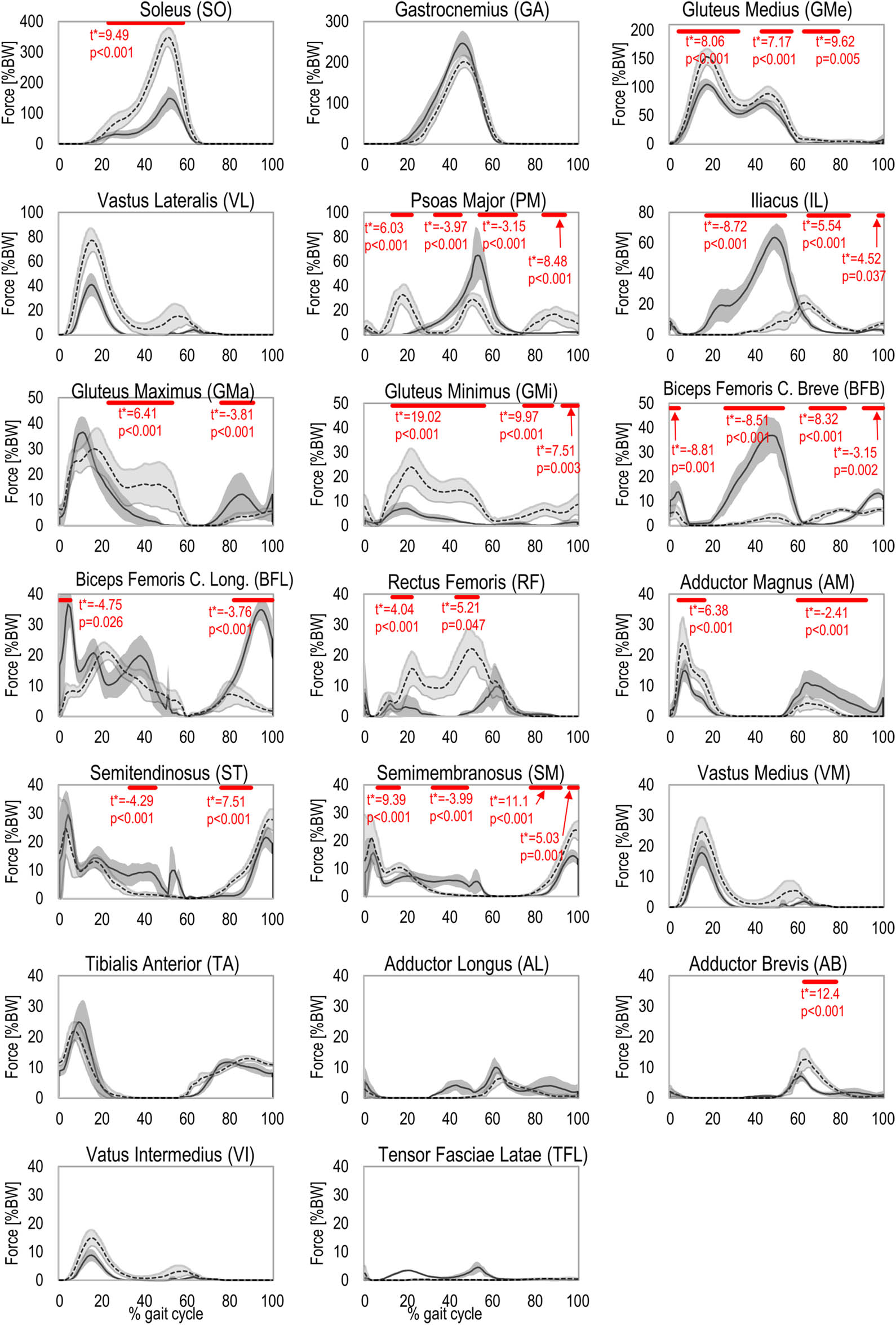
Figure 1
Time waveforms (mean and standard deviation) of the active muscle force for the 20 muscles of the lower limb, obtained using two standard models in the AnyBody Modeling System, i.e. TLEM 1.1 (dashed line) and TLEM 2.0 (solid line). Red bars denote significant differences (SPM{t}, p < 0.05), with peak t* (t max) values shown for each region.
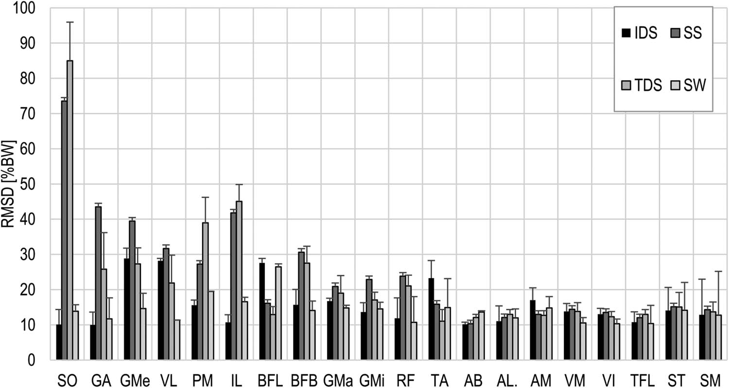
Figure 2
Mean RMSD for the comparison of muscle forces between the TLEM 1.1 and TLEM 2.0 models for four periods (IDS – initial double stance, SS – single stance, TDS – terminal double stance, SW – swing phase). Error bars represent one standard deviation. Abbreviations for muscle names are listed in Figure 1.
For all muscles, differences in active muscle force can be observed. Significant differences between the analysed models were observed for the muscles stabilising the pelvis and controlling movement in the hip joint. For the gluteus medius, three significant time ranges were observed (4–32%GC, 43–57%GC, 58–80%GC) with higher muscle force values obtained for the TLEM 2.0 model (t max = 9.62, p < 0.001). The RMSD for this muscle reached even 39.47%BW in the single stance phase. In the case of the gluteus maximus, both a decrease (28–51%GC, t max = 6.41, p < 0.001) and an increase (77–87%GC, t max = −3.81, p < 0.001) in muscle force were observed in TLEM 2.0 compared to TLEM 1.1. For the iliacus (t max = −8.72, p < 0.001) and psoas major (t max = 8.48, p < 0.001), the highest RMSD values were observed for the terminal double stance phase, 45%BW and 40%BW, respectively. For the rectus femoris (t max = 5.21, p = 0.047), smaller differences were noted (RMSD up to 25.04%BW in the single stance phase). In the case of the soleus, playing a crucial role in the stance phase, significant differences were observed in 23–59%GC (t max = 9.49, p < 0.001), with RMSD of 73.53%BW in the single stance phase and 83.96%BW in the terminal double stance phase.
It is worth noting that not all analysed muscles showed significant differences between the models. In the case of several muscles, the force waveforms obtained by use of both models were similar, but usually differences in the maximum values of the active force were observed (e.g. vastus muscles).
3.2. Joint reaction forces
Waveforms of particular components of the joint reaction forces in the hip, knee and ankle obtained using both TLEM 1.1 and TLEM 2.0 models are presented in Figure 3. Differences in joint reaction force were observed in all analysed directions, which was confirmed by both SPM{t} analysis (Figure 3) and RMSD values (Figure 4).
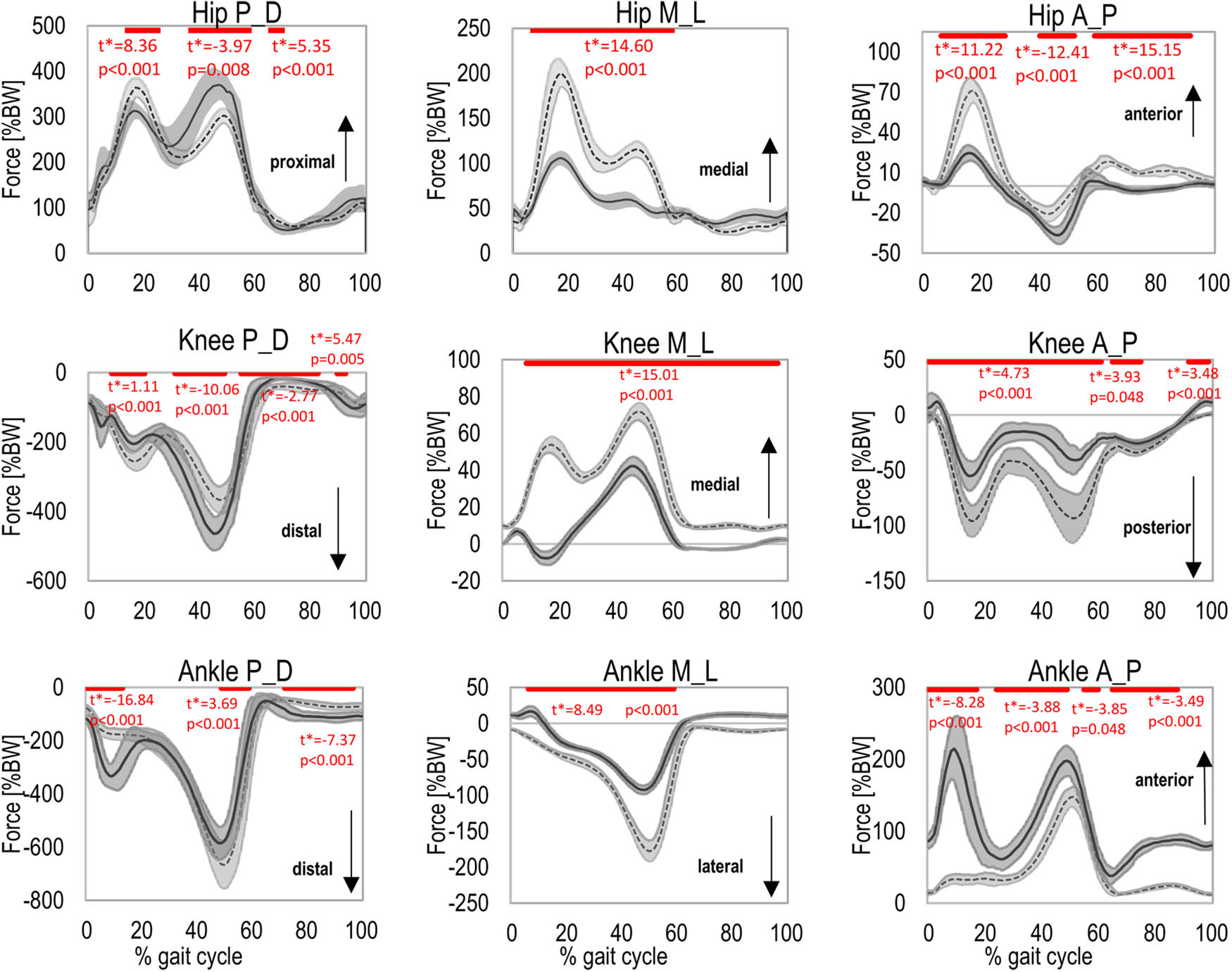
Figure 3
Time waveforms (mean and standard deviation) of the joint reaction force components for: (a) hip joint, (b) knee joint, (c) ankle joint (P_D – proximal [+] - distal [−]; M_L – medial [ +] - lateral [−]; A_P – anterior [ +] - posterior [−]). A comparison of the results obtained using the two standard models in the AnyBody Modeling System (TLEM 1.1 [dashed line] and TLEM 2.0 [solid line]) is shown. Red bars denote significant differences (SPM{t}, p < 0.05), with peak t* (t max) values shown for each region.
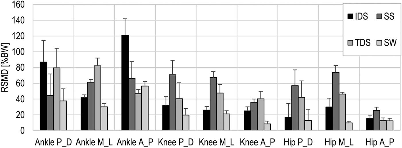
Figure 4
Mean RMSD for the comparison of joint reaction forces components (P_D – proximal [ +] - distal [−]; M_L – medial [ +] - lateral [−]; A_P – anterior [ +] - posterior [−]) between the TLEM 1.1 and TLEM 2.0 model for four periods (IDS – initial double stance, SS – single stance, TDS – terminal double stance, SW – swing phase). Error bars represent one standard deviation.
3.3. Hip
Waveforms of the proximo-distal (P_D) component of the hip joint reaction force had a characteristic profile with two pronounced local maxima (16–17%GC and 45–47%GC). The highest value was observed earlier in TLEM 1.1 (420%BW at 16%GC) compared to TLEM 2.0 (402%BW at 47%GC). The SPM analysis confirmed significant differences in the P_D component force waveforms between models, including a model-dependent phase of gait cycle in which particular models predicted higher force values – TLEM 1.1 showed higher forces in the early stance phase, whereas around in the mid-stance the forces predicted by TLEM 2.0 exceeded those of TLEM 1.1 (RMSD up to 58%BW in the single stance phase). The antero-posterior (A_P) component of the hip joint reaction force showed three time ranges of significant differences between analysed models (6–28%GC, 39–52%GC, 59–92%GC, t max = 15.15, p < 0.001), where TLEM 1.1 generated higher force values in the anterior direction and TLEM 2.0 in the posterior direction (RMSD up to 32%BW in the single stance phase). In the case of the medio-lateral (M_L) component statistically significant differences can be observed throughout almost the entire stance phase (9–59%GC, t max = 14.60, p < 0.001) with RMSD exceeding 70%BW.
3.4. Knee
Results for the knee joint showed that the first and the second local maxima of proximo-distal (P_D) components occurred at similar times (15–17%GC and 45–47%GC), but their values differed – the first maximum was higher for TLEM 1.1 (RMSD up to 72%BW in the single stance phase), and the second for TLEM 2.0. The SPM analysis confirmed a significant difference in the time range of 31–49%GC (t max = −10.06, p < 0.001). In the case of medio-lateral (M_L) component (t max = 15.01, p < 0.001) as well as antero-posterior (A_P) component (t max = 4.73, p < 0.001), throughout almost the entire gait cycle higher values were observed for the TLEM 1.1 model, with the highest RMSD values of 68%BW (SS) and 40%BW (TDS), respectively.
3.5. Ankle
The waveform of the ankle joint reaction force differed between the analysed models, especially in the initial part of the stance phase. While two local maxima of the proximo-distal (P_D) components were visible in TLEM 2.0, these were hardly noticeable in TLEM 1.1. The SPM analysis confirmed that statistically significantly higher values for the TLEM 2.0 model were obtained at the beginning of the gait cycle for the P_D component (t max = −16.84, p < 0.001), with the highest RMSD reaching 87%BW in the initial double stance phase. The antero-posterior (A_P) component varied between models for almost the entire gait cycle (t max = −8.28, p < 0.001, RMSD up to 120%BW in the initial double stance phase). For TLEM 1.1, only one local maximum (156.38%BW in 52.42%GC) was observed, whilst for TLEM 2.0, two local maxima were visible (215.29%BW in 10.69%GC and 204.42%BW in 49.38%GC). Moreover, for the medio-lateral (M_L) component, higher values were observed more often for the TLEM 1.1 model compared to TLEM 2.0 (t max = 8.49, p < 0.001, RMSD up to 81%BW in the terminal double stance phase).
4. Discussion
In the present study, a comparison was made between results calculated using the same modelling system (AnyBody Modeling System), applying identical scaling and optimisation procedures, but using different MSKS models (TLEM 1.1 and TLEM 2.0). The obtained results answer the research questions and support the hypothesis that structural differences between TLEM 1.1 and TLEM 2.0 significantly influence muscle forces and joint reaction forces in the joints of the lower limb (hip, knee and ankle) calculated during gait. Thus, a more general discussion on the problem of reliability of the results of the numerical simulation of the MSKS, and their dependency on the modelling methodology, can be provided.
Several studies have highlighted differences between the results obtained using various MSKS modelling systems (OpenSim, MATLAB, AnyBody) [14–17,19,21,37]. The authors of previous studies noted that the results of the numerical analyses can be influenced not only by different geometrical models, but also by scaling or optimisation procedures. In order to eliminate the latter two factors, in the present study a comparison was made between results calculated using the same modelling system (AnyBody Modeling System), applying identical scaling and optimisation procedures, but using different MSKS models (TLEM 1.1 and TLEM 2.0). Such a comparison, which is missing in the current literature, seems to be necessary for a better understanding of the results obtained from the numerical simulation and to facilitate the use of MSKS modelling in future studies. A comparison of TLEM 1.1 and TLEM 2.0 (Tables 1 and 2) shows that differences between them mainly relate to the geometry of the skeletal elements (pelvis and femur), the inclusion of fibula in the newer model, the different number of actuators and the changed paths of some important muscles.
Differences in model geometry influence the position of muscle attachment points, leading to variability in muscle moment arms, which was also confirmed by previous studies [12,28,29]. As a result, the values and time waveforms of the forces generated by individual muscle as well as joint reaction forces differ between the considered models [15,38]. Moreover, variations in bone geometry, the inclusion of additional structures (e.g. the fibula in TLEM 2.0), and updated muscle paths can lead to altered muscle activation strategies and load distribution during gait. This was also highlighted by Modenese and Renault [39], who demonstrated that accurate representation of bone geometry is essential for reliable modelling of the MSKS, and by Abdullah et al. [10], who emphasised the importance of selecting an appropriate model based on the purpose of biomechanical analysis. Our findings confirm that even within the same computational environment (AnyBody), switching between MSKS models can result in substantial discrepancies in outcomes, which is crucial for data comparison across studies.
The results obtained in this study confirmed that replacing the TLEM 1.1 with the TLEM 2.0 model leads to significant differences in both muscle force and joint reaction force time waveforms, especially during single stance and terminal double stance phases. Such differences may influence the biomechanical interpretation of muscle function and joint loading during gait analysis. The greatest discrepancies were observed in the muscles stabilising the pelvis (e.g. gluteus medius), in the hip flexors (iliacus, psoas major) and in the muscle responsible for push-off and lower limb stabilisation during the stance phase (soleus). The TLEM 2.0 model predicted lower force values for the gluteus medius, gluteus minimus and soleus, and higher force values for the iliacus and psoas major. Lower forces for hip abductor muscles during the stance phase suggest altered mechanical requirements for pelvic stabilisation in the coronal plane, which may result from differences in muscle paths and moment arms between the models. Lower forces for soleus may indicate a different distribution of plantar flexor load during the stance phase. In contrast, higher force values for the iliacus and psoas major during the terminal double stance phase suggest a greater contribution of hip flexors in preparing for swing. SPM{t} analysis (Figure 1) and RMSD values (Figure 2) confirmed significant differences in the activity of these muscles between the results obtained by use of particular models, suggesting that changes in the geometry of the model affect these muscle function estimation obtained during gait numerical simulation. Such results confirm the high sensitivity of musculoskeletal models to changes in their geometrical structure that may affect evaluation of the pelvic stabilisation and lower limb balance [28,29,37]. Similar discrepancies were observed when comparing simulation results performed in different modelling environments, such as AnyBody and OpenSim. Trinler et al. [14], when comparing different modelling systems (OpenSim and AnyBody), observed significant differences in muscle force waveforms for biceps femoris (short head), gastrocnemius and soleus (mainly during stance phase). Weinhandl and Bannet [12] showed that more accurate modelling of muscle paths improves muscle moment arms and thus better reflects the actual muscle force values. Research by de Pieri et al. [29] also pointed out that taking into account muscles wrapping around patient bones has a significant influence on loadings acting in the MSKS. These studies show that even minor model differences can influence muscle force predictions, in agreement with the present results. In particular, the greater forces generated by the gluteus muscles in the TLEM 2.0 model can be explained by the modified paths of these muscles, which increase their mechanical contribution to pelvic stabilisation [29]. A similar effect was described by Ismail and Lewis [26], who pointed out that changes in the orientation of the pelvis influence the functioning of these muscles. In contrast, slight differences in muscle force values were noted for the vastus muscles, where muscle paths remained unchanged between models (TLEM 1.1/TLEM 2.0) [28]. This indicates that the influence of changes between TLEM 1.1 and TLEM 2.0 is selective and primarily affects muscles with more complex structures or altered geometrical patterns.
The analysis of reaction forces in the joints revealed significant differences between the TLEM 1.1 and TLEM 2.0 models in the medio-lateral (M_L) direction, primarily during the stance phase. These differences were observed in both the SMP{t} analysis (Figure 3) and the RMSD values (Figure 4). Lower values of the medio-lateral component of the hip joint reaction forces observed in the TLEM 2.0 model during stance phase were associated with lower forces for the gluteus medius and the gluteus minimus, suggesting more effective mechanical conditions for hip abductor function and a reduced need for active pelvic stabilisation. This may indicate that the TLEM 1.1 model overestimated hip joint loading in the coronal plane. In the proximal-distal (P_D) and anterior-posterior (A_P) directions, smaller discrepancies were observed. The results obtained indicate that changes in the model structure affect not only the values of the forces, but also their entire time waveforms, which are consistent with the results of previous studies [12,14,28,29]. Improvements in muscle wrapping and attachment point, as reported by de Pieri et al. [29], or changes in muscle parameters between modelling systems, affect both the values and direction of joint reaction forces.
It is also worth noting that the earlier TLEM 1.1 model has been replaced by the updated TLEM 2.0 dataset, suggesting the need for continuous development and anatomical improvement of models [10,29,37,39]. Importantly, TLEM 2.0 was specifically designed to facilitate integration with imaging-based scaling techniques, which enable high anatomical fidelity [28]. de Pieri et al. [29] reported that refining the geometry of the muscles using MRI scans improved hip contact force predictions by approximately 17% and reduced root-mean-square error significantly (from ∼0.359*BW to 0.298*BW). These results suggest a closer match between the internal forces predicted by the model and experimental measurements, confirming the clinical utility of TLEM 2.0 in applications where anatomical precision is critical.
In summary, this study provides valuable insight into the differences in biomechanical results obtained from numerical simulation performed with the use of different MSKS models within the same modelling environment. It highlights the importance of an accurate musculoskeletal model for achieving consistency in muscle force and joint reaction force estimation. These results underline the need to improve musculoskeletal models and to develop more advanced methods for model personalisation. Modenese and Renault [39] pointed out that the use of personalised musculoskeletal models is a cumbersome and time-consuming task. However, this approach becomes particularly important in the case of pathological changes in the MSKS, such as those observed in cerebral palsy [6].
Furthermore, it is highly probable that future research should include verification of models using experimental data, which will allow for the assessment of the accuracy of the obtained simulation results [3].
In recent years, there has been a growing use of statistical parametric mapping (SPM) analysis in biomechanical gait studies. Studies by Mestanza Mattos et al. [40] and Yona et al. [32] exemplified the broad applicability and precision of SPM in gait analysis, from diagnosing movement disorders to enhancing athletic performance. In the context of this study, SPM proves particularly valuable, as it enables the detection of subtle, time-dependent differences in muscle and joint force outputs between the analysed musculoskeletal models that traditional gait analysis methods based on discrete data points or averages may not capture.
This study has several limitations, including a limited sample size of 20 individuals, who walked with preferred velocity. It remains unclear how walking speed would affect generic models with Hill-type muscles in both models, which should be addressed in further research. Another limitation of this study is the use of group-level analysis, as inter-subject variability in the model effect was not evaluated. Furthermore, muscle activation patterns in gait analysis calculated using both models should be compared to measured electromyographic muscle activations and to assess the extent to which the newer model has improved compatibility with experimental data.
5. Conclusions
The geometrical structure of the MSKS model has a significant influence on the muscle forces and joint reaction forces predicted by numerical simulation. Comparing the TLEM 1.1 and TLEM 2.0 models available in the AnyBody Modeling System, the largest differences were observed in pelvic stabilisers, hip flexors and muscles responsible for push-off and lower limb stabilisation during stance phase. The TLEM 2.0 model predicted lower forces for the hip abductor during stance phase and higher forces for the psoas major and iliacus during terminal double stance phase. These results were reflected in lower values of the medio-lateral component of the hip joint reaction forces, suggesting altered mechanical requirements for pelvic stabilisation and hip joint loading. Overall, the obtained results confirm the importance of the geometrical model of the MSKS used to simulate human movement in the context of the reliability of the results obtained this way. They also emphasise the need for careful selection of the musculoskeletal model in simulation studies, as even minor geometric discrepancies can significantly alter the predicted biomechanical results.
Acknowledgements
The research was conducted as a part of the Project WZ/WM-IIB/5/2026 and financed with the use of funds for science from the Polish Ministry of Science and Higher Education.
Funding information
Faculty of Mechanical Engineering (Wydział Mechaniczny) at the Bialystok University of Technology (Politechnika Białostocka) in Poland (WZ/WM-IIB/5/2026).
Author contributions
JS, SP – study conception and design, methodology, JS – manuscript drafting; JS - data acquisition, and analysis; JS, SP – critical revision, and SP – supervision. All authors approved the final version of the manuscript and accept responsibility for the work.
Conflict of interest statement
No conflict of interest to report.