
Table 1. Aircraft instrumentation used in the study
(diameter >10 nm)TSI 30101 scm−3Aerosol size distribution
15 channels (0.3<diameter <20 µm)GRIMM 1.1086 scm−3Wind speed and directionINS/Noseboom probe0.1 sm s−1TemperaturePt100, Meteolab1 s°CDew pointDew point mirror, Meteolab1 s°C
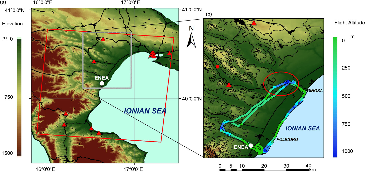
Fig. 1
(a) Map of the experiment region. The red square indicates the domain of the 1 km×1 km 3-D meteorological field used to calculate the high-resolution back-trajectories. Red triangles and black spots show, respectively, the chimney stacks and the urban areas; the main roads are indicated by black lines. The white circle indicates the ENEA Research Centre of Trisaia. (b) The paths of the 17 June morning and afternoon flights are shown on a detailed map of the study area. The red circle shows the location of the air quality station at Ferrandina. The red oval indicates the inland area sampled in the afternoon flight and discussed in Section 3.3.2.
Table 2. Time, altitude and distance from the airstrip are indicated for the starting and ending points of each profile of the morning (XXAM) and afternoon (XXPM) flights on 17 June
Table 3. RAMS parametrisations used in this study
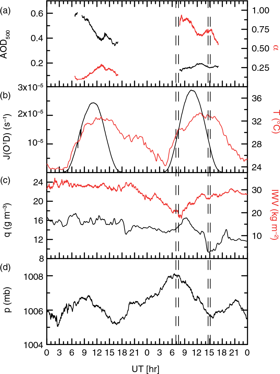
Fig. 2
Time series of (a) aerosol optical depth (AOD500) and Ångström exponent (α), (b) ozone photolysis frequency [J(O1D)] and surface temperature (T), (c) surface absolute humidity (q) and integrated water vapour (IWV), (d) surface pressure (P) for 16 and 17 June. Black curves indicate AOD500, J(O1D), q and P, while red curves α, IWV and T. Time intervals of morning and afternoon flights are indicated by dashed lines.
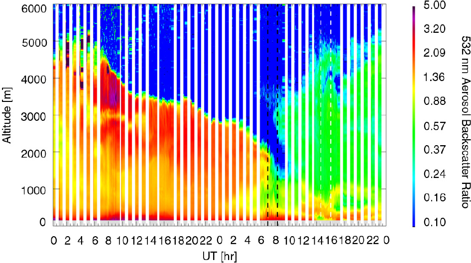
Fig. 3
Time evolution of the aerosol backscatter ratio profile on 16 and 17 June, as measured by the LIDAR from the ENEA Research Centre. The time intervals of the morning and afternoon flights are indicated by dashed lines.
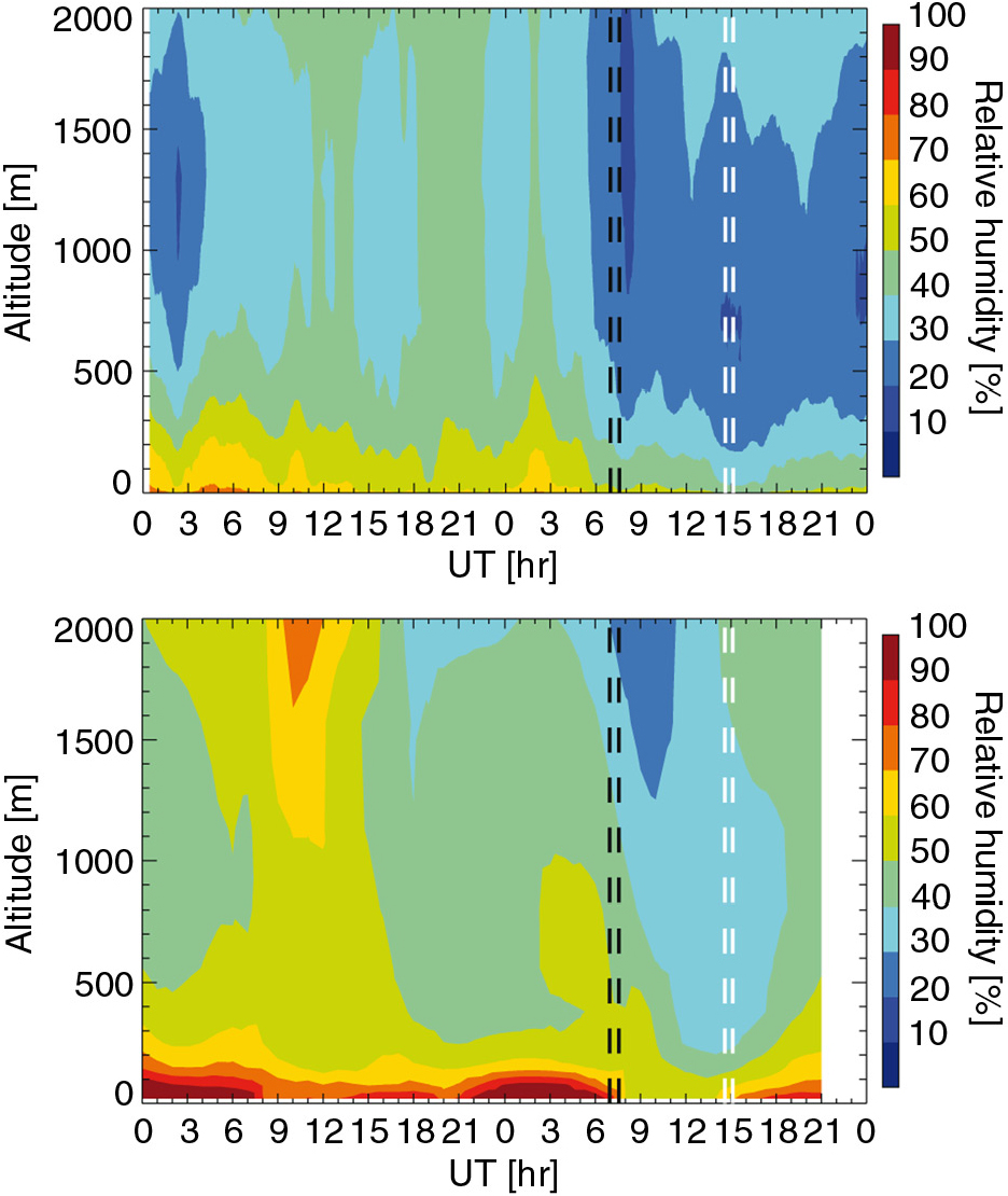
Fig. 4
Time evolution of the relative humidity profiles on 16 and 17 June, as measured by the HATPRO from the ENEA Research Centre (upper panel) and simulated by RAMS at 1 km horizontal resolution (lower panel). The time intervals of the morning and afternoon flights are indicated by black and white vertical dashed lines, respectively.
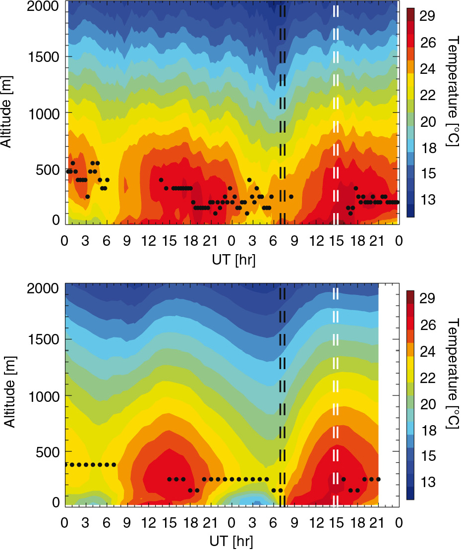
Fig. 5
Time evolution of the temperature profile on 16 and 17 June, as measured by the HATPRO from the ENEA Research Centre (upper panel) and simulated by RAMS at 1 km horizontal resolution (lower panel). Black dots indicate the altitude of the temperature maximum for cases in which a temperature inversion is present. The time intervals of the morning and afternoon flights are indicated with black and white vertical dashed lines, respectively.
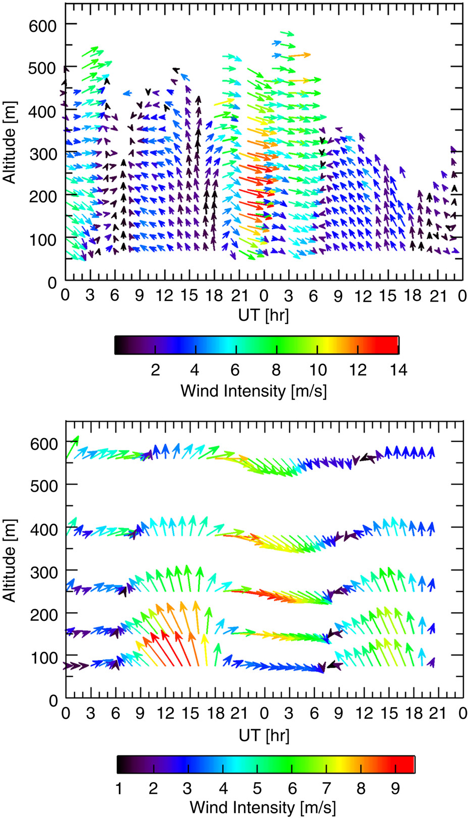
Fig. 6
Time evolution of the measured horizontal wind profile on 16 and 17 June, as measured by SODAR (upper panel) from the ENEA Research Centre and simulated (lower panel) at 1 km horizontal resolution.
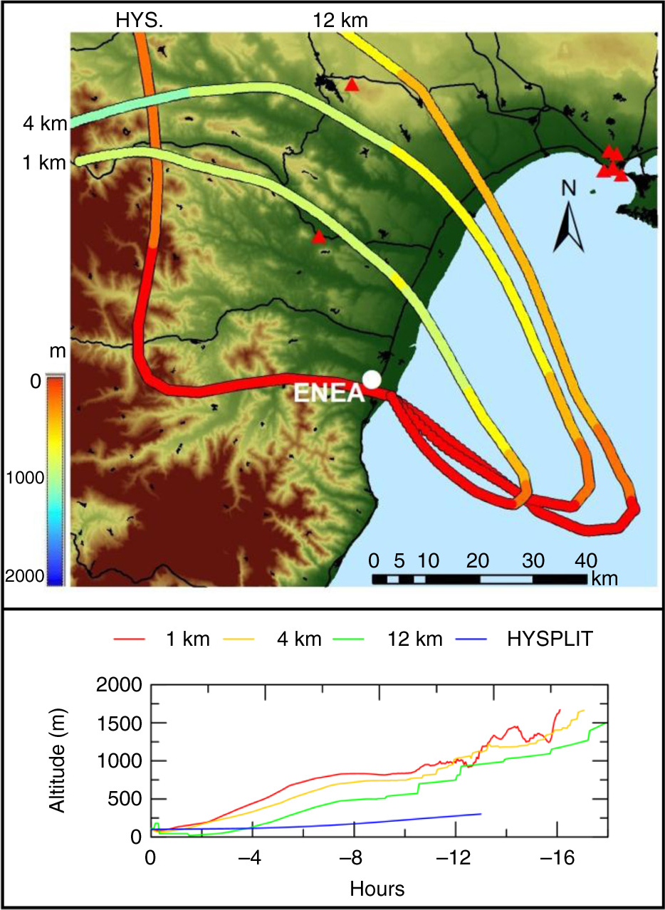
Fig. 7
Upper panel: back-trajectories arriving at the altitude of 100 m during the first afternoon ascent (A1PM) calculated using M-TraCE with 3-D meteorological field at 1 km, 4 km and 12 km horizontal resolution, and using HYSPLIT with NCEP/NCAR global reanalysis. Lower panel: time evolution of the back-trajectories’ altitude.
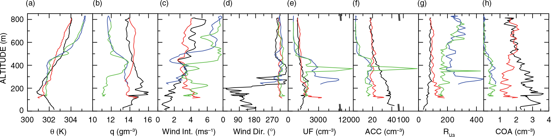
Fig. 8
Vertical profiles of (a) potential temperature, (b) absolute humidity, (c) wind intensity, (d) wind direction, (e) UF, (f) ACC, (g) R U3 and (h) COA during A1AM (black curves), D1AM (red), A2AM (blue) and D2AM (green).
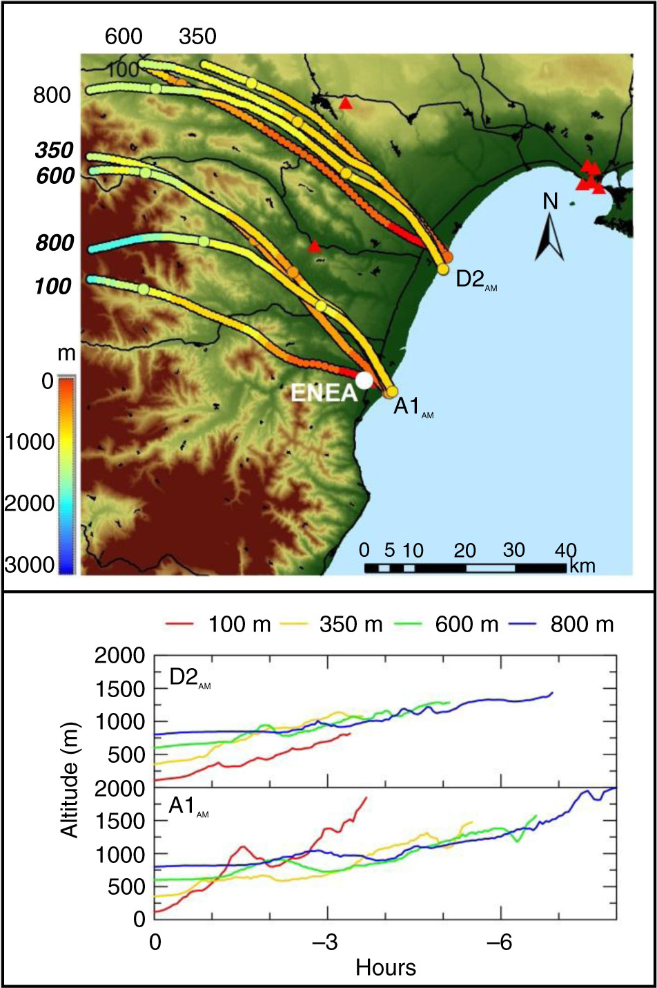
Fig. 9
Upper panel: back-trajectories arriving at 7:00 UT at 100, 350, 600 and 800 m of the A1AM and D2AM profiles. Bold italic characters refer to the A1AM profiles. Three-hour intervals along the trajectories are marked with circles. Lower panel: time evolution of the airmass altitude along the trajectory.
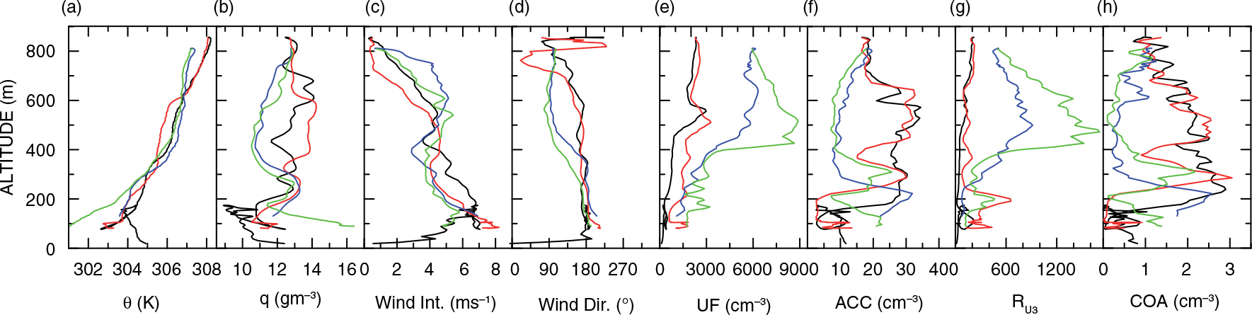
Fig. 10
Vertical profiles of (a) potential temperature, (b) absolute humidity, (c) wind intensity, (d) wind direction, (e) UF, (f) ACC, (g) R U3 and (h) COA during A1PM (black curves), D1PM (red), A2PM (blue) and D2PM (green).
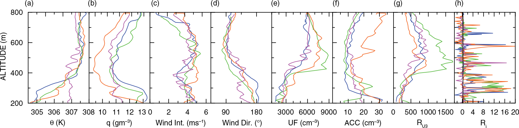
Fig. 11
Vertical profiles of (a) potential temperature, (b) absolute humidity, (c) wind intensity, (d) wind direction, (e) UF, (f) ACC, (g) R U3 and (h) gradient Richardson number during A2PM (blue curves), D2PM (green curves), A3PM (orange curves), D3PM (purple curves). Vertical smoothed profiles of potential temperature and wind intensity and direction used to calculate R i are shown. The value of R i,c is marked by a vertical black line in panel (h).
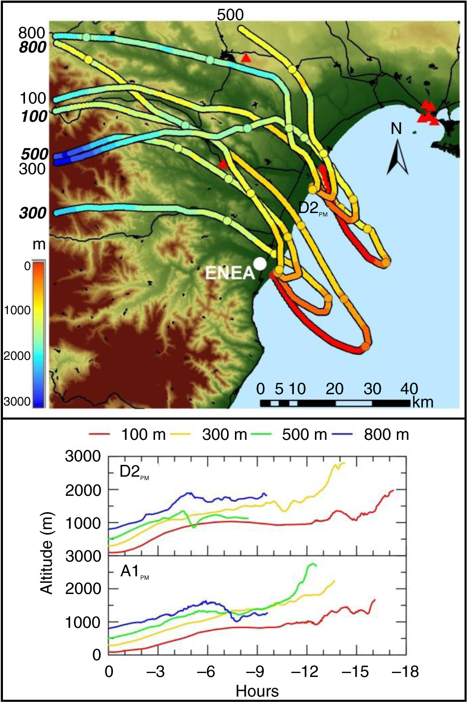
Fig. 12
Upper panel: back-trajectories arriving at 15:00 UT at 100, 300, 500 and 800 m during the A1PM and D2PM profiles. Three-hour intervals along the trajectories are evidenced by larger circles. Bold italic characters refer to the A1PM profiles. Lower panel: time evolution of the airmass altitude along the trajectories.