
1. Introduction
Atmospheric aerosols play an important role in the Earth climate, representing together with clouds, the largest uncertainty in climate change assessment (Boucher et al., 2013). In addition, aerosols may affect the human health (Bräuner et al., 2007; Brook et al., 2010; Dominici et al., 2014).
In the last decades, the scientific community has dedicated a large effort to the understanding of the aerosol processes, and the knowledge of its role in the climate system (Haywood and Boucher, 2000) and in air quality (Monks et al., 2009) has substantially increased. Nevertheless, large uncertainties affect the full understanding of the aerosol direct and indirect effects, mainly due to the large variability of the aerosol properties and the difficulty to properly characterise natural and anthropogenic sources. It is extremely difficult to provide an accurate description of the aerosol spatial and temporal distribution at the regional scale, particularly for particles in the submicron size range. These factors critically influence the performance of air quality modelling.
The Mediterranean is a nearly closed sea, whose surrounding regions are characterised by a very complex orography which affects atmospheric dynamics on different scales. The Sahara desert and the basin itself are the main sources of natural aerosols, mineral dust and sea salt, respectively. Due to the high population density in the coastal regions, anthropogenic emissions also play a large role. Thus, different aerosol types of natural and anthropogenic origin (urban and industrial plumes, fires, emissions from ships), often mixed in various ways (Lelieveld et al., 2002; Kallos et al., 2007; Monks et al., 2009), are found over the Mediterranean.
Currently, most of the knowledge on the Mediterranean aerosol characteristics is derived from ground-based in situ and remote sensing measurements, generally made at coastal sites, and from satellite observations. Few long-term time series of in situ observations are available and provide precious information on the physical and chemical properties of particles of different size (Asmi et al., 2011; Cusack et al., 2013; Kopanakis et al., 2013). On the other hand, ground-based and satellite remote sensing observations provide columnar and, in some cases, vertically resolved properties only for particles larger than few hundreds of nanometres, since current remote sensing techniques are not suited to measure the submicron particles’ properties.
Studies of the atmospheric vertical structure and chemical composition of the Mediterranean region were started at the end of the 1980s (Millán et al., 1997, 2000), and they have shown the high complexity of coastal areas. More recently, Palau et al. (2005) have highlighted the importance of the different meteorological scales for air quality studies in the coastal region, showing how surface observations do not always reflect the vertical distribution in the atmospheric column.
In this respect, airborne observations of aerosol microphysical and optical properties, although not continuous and often focused on specific events, constitute the only method to accurately describe the vertical variability of the aerosol properties on scales ranging from local to regional, in particular for small size particles. These data sets constitute important basis for process studies and model validation. Unfortunately, airborne campaigns are rare, due to the high costs and the difficulty of airborne observations.
This work presents and discusses ground-based and airborne measurements of the atmospheric and aerosol vertical structure made during MORE, the Marine Ozone and Radiation Experiment carried out in June 2010 in a coastal area along the Ionian Sea, in Southern Italy. The study is focussed, in particular, on an event in which dust transport, descent of dry mid-tropospheric air and sea breeze circulation coincide. Evidence of local pollution and, possibly, nucleation phenomena, was found during the same event. Two flights with the Karlsruhe Institute of Technology (KIT) Enduro ultralight instrumented aircraft were carried out on 17 June, providing a picture of the complexity of the atmospheric dynamical structure and of the vertical aerosol distribution. The two flights, one during the morning and one in the afternoon, followed a nearly identical path, providing the rare possibility to observe by in situ and remote sensing techniques the evolution of the meteorological and aerosol profiles on the daily timescale under the influence of large-scale advection and local sea breeze transport phenomena.
The analysis is complemented with results from a high-resolution regional atmospheric model, used to calculate airmass trajectories which support the interpretation of the measurements. The model capability to reproduce the meteorological observations for different model spatial resolutions is discussed.
The field observations and model analyses are used for the main objectives of the present study:
discuss the variability and complexity of the atmospheric thermodynamic vertical structure and aerosol distribution in a Mediterranean coastal environment with complex orography;
highlight the role of high-resolution meteorological fields for the understanding of transport phenomena in this type of environment.
2. Measurements and methodology
2.1. The MORE campaign
The MORE airborne campaign was aimed at investigating the vertical distribution of aerosol and ozone in a rural coastal area with complex orography. The campaign was supported by the EUFAR (European Fleet for Airborne Research) project and took place in conjunction with the validation campaign of the MINNI (National Integrated Assessment Modeling System for Policy Making, Italy, www.minni.org) project in Southern Italy in May–June 2010. The airfield was located less than 2 km from the ENEA (Italian National Agency for New Technologies, Energy and Sustainable Economic Development) Trisaia Research Center (40.16°N, 16.63°E), where a large set of ground-based and remote sensing instruments was deployed for the campaign (e.g. Malaguti et al., 2013, 2015; Mateos et al., 2014, 2015).
Airborne measurements were carried out using the Enduro KIT ultralight aircraft, which carries up to 80 kg of scientific payload (Junkermann, 2001). Thanks to the low flight speed (~20 ms−1) and the possibility to fly at low altitudes, the Enduro KIT is particularly suited to study the lowest levels of the atmosphere and the horizontal variability over local to regional spatial scales. The aircraft was equipped with sensors to measure meteorological parameters, aerosol and ozone concentrations, aerosol size distribution, ground temperature, and down- and up-welling solar radiation. Table 1 reports the main characteristics of the aerosol and meteorological instrumentations used in this study.
Table 1. Aircraft instrumentation used in the study
(diameter >10 nm)TSI 30101 scm−3Aerosol size distribution
15 channels (0.3<diameter <20 µm)GRIMM 1.1086 scm−3Wind speed and directionINS/Noseboom probe0.1 sm s−1TemperaturePt100, Meteolab1 s°CDew pointDew point mirror, Meteolab1 s°C
Among the ground-based instruments installed at the ENEA Research Centre of Trisaia, hereinafter ENEA, a visible Multi Filter Rotating Shadow band Radiometer, MFRSR (Harrison et al., 1994), a Diode Array Spectrometer, DAS (Mateos et al., 2015), an elastic backscatter LIDAR (Di Iorio et al., 2009), a Humidity And Temperature microwave PROfiler, HATPRO (Rose et al., 2005), and a three-axis, monostatic Doppler SODAR (Rao et al., 2004) provided observations used in this study.
The aerosol optical depth (AOD) at different wavelengths in the visible and near infrared and the Ångström exponent (α) were derived from continuous MFRSR measurements. The Ångström exponent was calculated from the AOD at 415 and 869 nm and provides an indication of the columnar aerosol size distribution; high and low values of α indicate, respectively, the dominant effect of fine and coarse particles. The ozone photolysis frequency, J(O1D), is estimated from DAS observations (Casasanta et al., 2011) and provides an indication of the atmospheric photochemical activity. LIDAR measurements were routinely made with one 15-minute interval of continuous measurements per hour throughout the campaign, providing the temporal evolution of the aerosol vertical distribution. In addition, continuous LIDAR observations were carried out during the flights and when interesting atmospheric conditions occurred. The laser backscattered radiation at 532 nm is mainly sensitive to aerosol particles in the accumulation and coarse mode. The HATPRO provided continuous tropospheric profiles of humidity and temperature as well as the integrated water vapour (IWV) amount. Continuous wind profiles up to ~450 m were obtained by SODAR during the whole campaign.
Vertical in situ profiles of potential temperature, absolute humidity, wind intensity and direction are used to describe the boundary layer thermodynamical structure and variability. Aerosol number concentrations in three size ranges are used to describe the aerosol distribution of the ultrafine (UF), accumulation (ACC) and coarse (COA) particles and are derived from measurements of the airborne condensation particle counter and optical particle counter (OPC). In this study, UF, ACC and COA indicate the number concentration of particles with optical diameters, hereinafter D, in the ranges 0.01–0.3, 0.3–1.0, and >1.0 µm, respectively. No measurements of the UF particle's size distribution were available on board the aircraft during MORE. Thus, only limited information is available on possible new particles formation (NPF) events. The reader is reminded that often the accumulation mode is defined as the one comprising particles with diameters between 0.09–0.1 and 1 µm (Kulmala et al., 2004, Asmi et al., 2011); we use a different lower limit, based on the available observations, for this mode.
The ratio between UF and the concentration of particles with 0.3 < D<0.4 µm (the smallest class measured by the OPC) is defined as the parameter R U3, and is used to investigate the evolution of UF with respect to the smaller fraction of the accumulation mode. R U3 provides a qualitative indication on the relationship between UF and accumulation mode particles. Asmi et al. (2011) discussed ground-based measurements of submicron aerosol number concentrations made at 24 European sites belonging to the EUSAAR (European Supersites for Atmospheric Aerosol Research) and the GUAN (German Ultrafine Aerosol Network) networks. Based on measurements of dried aerosol electrical mobility diameter, they show that the Aitken (0.03<D<0.1 µm) and the accumulation (D>0.1 µm) modes are generally related; the correlation is particularly strong at the Mediterranean site of the EUSAAR network, the station of Finokalia on Crete.
Several studies suggest that the mixing of different airmasses determined by turbulence is one of the processes favouring the formation of new particles (Bigg, 1997; Nilsson et al., 2001; Hellmuth, 2006; Wehner et al., 2010). To investigate this possibility, the gradient Richardson number, R i, is calculated and used as an indicator of dynamic stability conditions or turbulence. R i is defined as the ratio between buoyancy forces and wind shear, and it is calculated as a function of altitude as follows:
where g is the gravity acceleration, θ is the potential temperature and U is the horizontal wind intensity. Averages of θ and U over 4 m vertical intervals are used to calculate the R i profiles. Turbulence can develop when R i is below the critical Richardson number, R i,c=0.25, while it is damped for R i>1. There are however indications that, once initiated, a turbulent flow can exist up to R i~1, due to the presence of hysteresis phenomena (Balsley et al., 2008).
2.2. Study area and flight pattern on 17 June 2010
Figure 1 shows orography, main towns and point emission sources in the region of the MORE campaign. The investigation area is part of the Basilicata region in Southern Italy, on the large Gulf of Taranto in the Ionian Sea. The region is dominated by the Appennino Lucano mountain range, whose highest peak is mount Pollino (2248 m), located about 50 km Southwest of ENEA. A relatively flat region, the Metaponto plain, exists North of ENEA, along the Ionian coast, while lower altitude mountains, between 500 and 1000 m, characterise the sector further North. The alluvial plain of Metaponto is characterised by various valleys which run perpendicular to the coastline and play an important role in the local circulation, interacting with the mountain–sea breeze regime. The airfield is located in a rural area, 2 km East of ENEA and at ~3 km from the coastline. Basilicata has one of the lowest population densities in Italy (~57 residents km−2) and is characterised by low anthropogenic emissions. The most populated town of the area is Policoro (16 000 inhabitants), located ~4 km North of the airfield (see Fig. 1b). The red triangles displayed in Fig. 1 show the main industrial sources of emissions. The largest and more industrialised area is in proximity of the city of Taranto, 60 km North-East of ENEA, with significant urban (~200 000 inhabitants) and large industrial emissions. In summer, due to the prevalence of a land–sea circulation, the plumes from Taranto only occasionally influence the study area (Gariazzo et al., 2007). The average surface aerosol concentration is generally low, as expected for a rural site. The 2009 annual average PM10 at the air quality station closest to ENEA, in Ferrandina (Fig. 1b), was 17 µg m−3, with minimum and maximum hourly values, respectively, of 3 and 51 µg m−3 (www.arpab.it/aria/report/). The average PM10 and PM2.5 values measured at ENEA Trisaia during the MINNI campaign were 18.6±9.9 and 11.0±4.0 µg m−3, respectively (Malaguti et al., 2015).
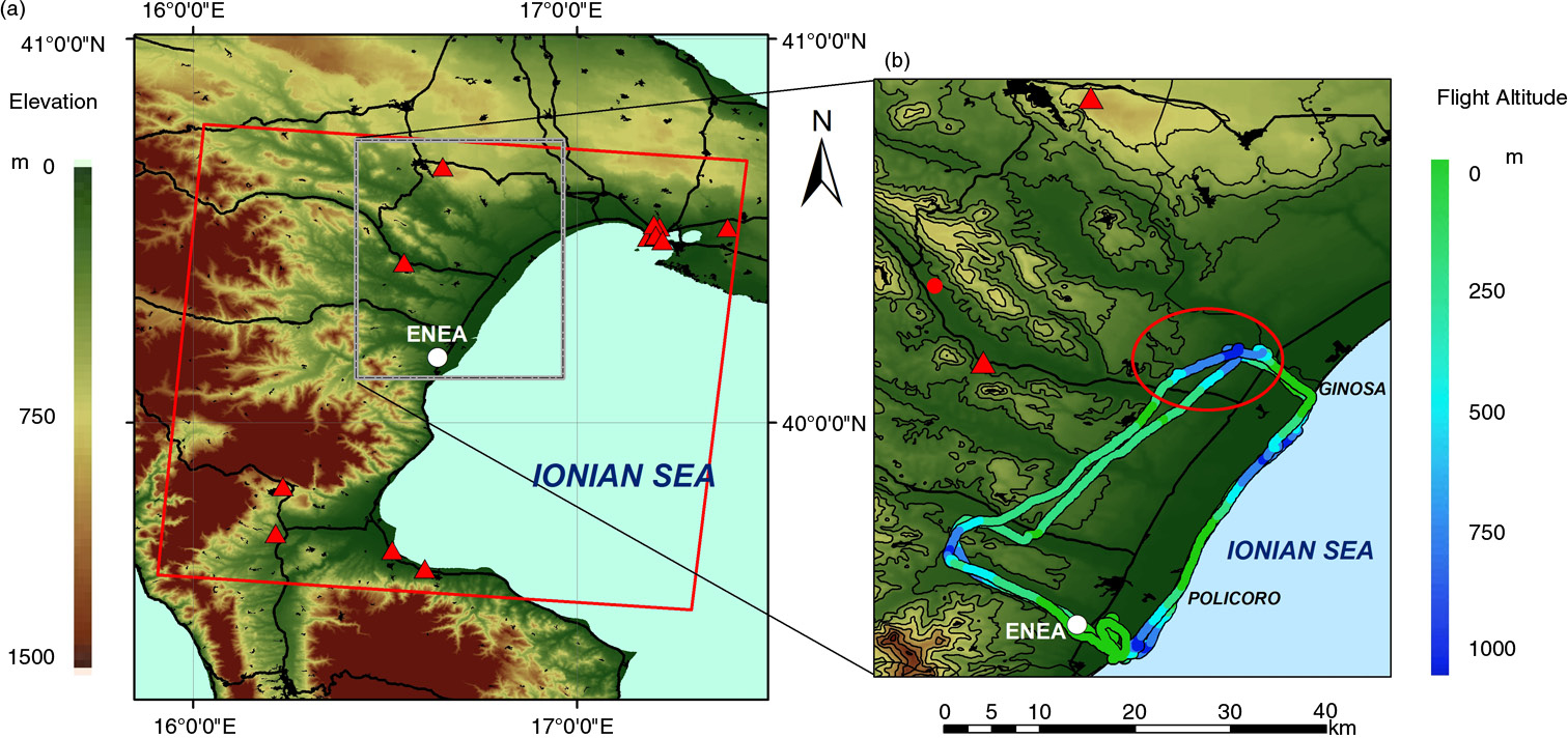
Fig. 1
(a) Map of the experiment region. The red square indicates the domain of the 1 km×1 km 3-D meteorological field used to calculate the high-resolution back-trajectories. Red triangles and black spots show, respectively, the chimney stacks and the urban areas; the main roads are indicated by black lines. The white circle indicates the ENEA Research Centre of Trisaia. (b) The paths of the 17 June morning and afternoon flights are shown on a detailed map of the study area. The red circle shows the location of the air quality station at Ferrandina. The red oval indicates the inland area sampled in the afternoon flight and discussed in Section 3.3.2.
\Twelve flights were performed from 12 to 26 June 2010. Typical flight patterns generally comprise a leg along the coastline, and an almost parallel leg about 20 km inland. The maritime section of the flights ended in proximity of Marina di Ginosa (6000 inhabitants). The first part of each flight was generally characterised by a first ascent–descent over the sea in the proximity of the shoreline, close to the ENEA research centre. A second ascent–descent was made at the end of the longest lag, close to Marina di Ginosa. Thus, four vertical profiles were obtained for each flight along the coast over the altitude range between ~100 and ~900 m. In the return part, the ultralight aircraft generally flew at constant altitude. The paths of the morning and afternoon flights of 17 June are shown in Fig. 1b. Inland measurements are largely influenced by the local orography and local aerosol sources, and only the vertical profiles made along the coastline are discussed here. Thus, the data set consists of two ascending (A1AM, A2AM) and two descending profiles (D1AM, D2AM) in the morning, between 06:58 and 07:26 UT, and two ascending (A1PM, A2 PM) and two descending (D1PM, D2PM) profiles in the afternoon between 14:36 and 15:07 UT. Table 2 summarises time and location of the vertical profiles, and horizontal distances from the airfield.
Table 2. Time, altitude and distance from the airstrip are indicated for the starting and ending points of each profile of the morning (XXAM) and afternoon (XXPM) flights on 17 June
2.3. Regional model and back-trajectory analyses
Back-trajectories were calculated to support the interpretation of the observations. Trajectory models constitute a useful and widely used tool to determine the airmass origin and history. For instance, they allow to establish source–receptor relationships of air pollutants (Salvador et al., 2010) and to identify pathways of desert dust transport (e.g. Meloni et al., 2007) and pollutants, such as ozone (e.g. Kuang et al., 2012).
For the purposes of this study, the Hybrid Single Particle Lagrangian integrated Trajectory model, HYSPLIT (Draxler and Rolph, 2014; Rolph, 2014), was run with the 3-D meteorological field of the NCEP/NCAR global reanalysis data archive (Kalnay et al., 1996), which has a horizontal resolution of 2.5°, 17 pressure levels from 1000 to 25 mb, and 6 hour time resolution. Due to the complex orography of the coastal region, the accuracy of back-trajectories based on low-resolution meteorological data, especially in proximity of the surface, is limited. Thus, high-resolution data and trajectories are preferable to better describe the evolution of the airmasses (Fleming et al., 2012), and additional trajectories were calculated from high-resolution meteorological fields.
Within the MINNI Atmospheric Modeling System (Mircea et al., 2014), meteorological fields are produced using the prognostic non-hydrostatic RAMS (Regional Atmospheric Modeling System) model, based on terrain following vertical coordinate system (Cotton et al., 2003). Simulations are made over nested domains (two-way nesting mode) and are carried out in nudging mode, that is, assimilating reanalysis fields during model runs; a forcing term is added to the dynamical equations, driving the model to follow more closely the meteorological observations. Reanalysis fields for the assimilation are produced using, as input data, ECMWF (European Centre for Medium-Range Weather Forecast) fields together with surface synoptic data (temperature, pressure and wind) from the WMO (World Meteorological Organization) network. For the purpose of the MINNI validation campaign, RAMS version 6.0 was run using four nested domains with horizontal resolutions of 48, 12, 4 and 1 km, respectively, and 35 irregularly spaced vertical levels, from the surface up to ~20 km. The parametrisations used in these simulations are summarised in Table 3. The 3-D atmospheric fields were produced at hourly intervals; the simulation at 1 km provides a reasonable description of the atmospheric state also in a domain with a complex orography (see Section 3.1.1).
Table 3. RAMS parametrisations used in this study
Back-trajectories were calculated from the 12, 4, and 1 km resolution fields using the M-TraCE (Module for Trajectories Calculation and statistical Elaboration) tool, recently developed in the frame of the MINNI modelling suite (Vitali et al., 2013). M-TraCE, whose computation algorithm is similar to that of HYSPLIT, takes advantage of the availability of the 3-D MINNI high-resolution meteorological database. The benefits of using 3-D meteorological fields with high spatial resolution have been recently discussed by Hernández-Ceballos et al. (2014), who used back-trajectories to study the transport of Olea pollen in Southern Spain.
In the following analysis, the two back-trajectory datasets, derived from HYSPLIT and from M-TraCE, are used to interpret the observations and to assess the role of the increased model spatial and temporal resolution.
3. Results
3.1. Ground-based observations
The evolution of AOD at 500 nm (AOD500), α, J(O1D), IWV, surface temperature (T), absolute humidity (q) and pressure (P) during 16 and 17 June is shown Fig. 2.
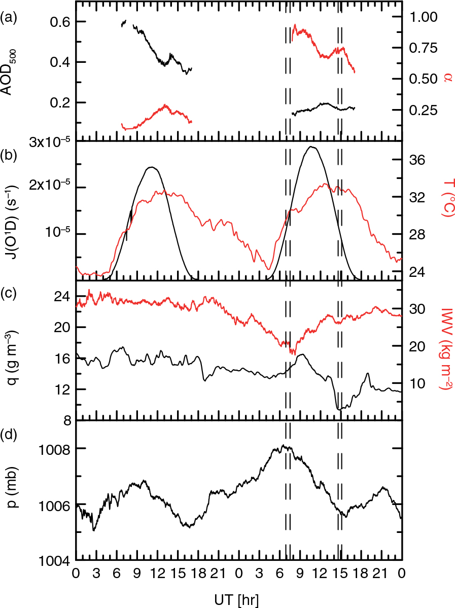
Fig. 2
Time series of (a) aerosol optical depth (AOD500) and Ångström exponent (α), (b) ozone photolysis frequency [J(O1D)] and surface temperature (T), (c) surface absolute humidity (q) and integrated water vapour (IWV), (d) surface pressure (P) for 16 and 17 June. Black curves indicate AOD500, J(O1D), q and P, while red curves α, IWV and T. Time intervals of morning and afternoon flights are indicated by dashed lines.
The AOD peaks during the morning of 16 June, with values as large as 0.6, associated with α values smaller than 0.2 (Fig. 2a). Pace et al. (2006) showed that the central Mediterranean cases with AOD500>0.15 and α<0.5 are dominated by desert dust, suggesting that considerable amounts of mineral dust were present on 16 June. Airmass trajectories (not shown) originate from North Africa and support this attribution. The presence of dust is related to a Saharan dust outbreak influencing the region since 10 June. During 17 June, AOD500 and α vary between 0.15–0.17 and 0.6–0.4, respectively, showing a strong reduction of dust load and columnar aerosol size with respect to the previous day. Almost no clouds were observed during the two days. June 17 was also characterised by an intense photochemical activity, as suggested by the high J(O1D) values, reaching 2.9 10−5 s−1 (Fig. 2b); the maximum J(O1D) values of the previous day are 16% lower, due to the attenuation of UV radiation induced by desert dust.
IWV shows a ~40% decrease from late 16 June to the morning of 17 June (Fig. 2c) and reaches the minimum value of ~17.5 kg m−2 around 8:00 UT on 17 June. The surface pressure shows a small 1 mb increase, as expected during subsidence phenomena, in correspondence with the 17 June morning flight (Fig. 2d). The pressure increase is superimposed to the semidiurnal cycle of the atmospheric tides. The surface temperature (Fig. 2b) is similar in the two days; the surface q displays a relevant decrease (36%) during the afternoon flight of 17 June, passing from 14.7 g m−3 at 13:12 to 9.4 g m−3 at 14:52 UT (Fig. 2c). A time shift of ~7 hours occurs between the minimum values of IWV and q.
The evolution of the aerosol vertical distribution, as derived from the LIDAR observations, during 16 and 17 June is shown Fig. 3. The figure displays the time–height evolution of the LIDAR backscatter ratio at 532 nm, here defined as the ratio between aerosol and molecular backscattering coefficients at 532 nm (i.e. the backscatter ratio is zero for a pure molecular atmosphere). A thick aerosol layer extending from the surface to 4–5 km altitude, with a maximum backscatter ratio of ~3.5 at about 3.5 km, was present on 16 June. LIDAR observations show the progressive reduction of the dust layer, which is replaced in the early morning of 17 June by an airmass with very low aerosol content.
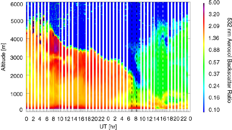
Fig. 3
Time evolution of the aerosol backscatter ratio profile on 16 and 17 June, as measured by the LIDAR from the ENEA Research Centre. The time intervals of the morning and afternoon flights are indicated by dashed lines.
The decrease of IWV (Fig. 2c) and relative humidity (Fig. 4) during the morning of 17 June suggests the arrival of a dry airmass, which also displays a low aerosol content, as detected by LIDAR (Fig. 3).
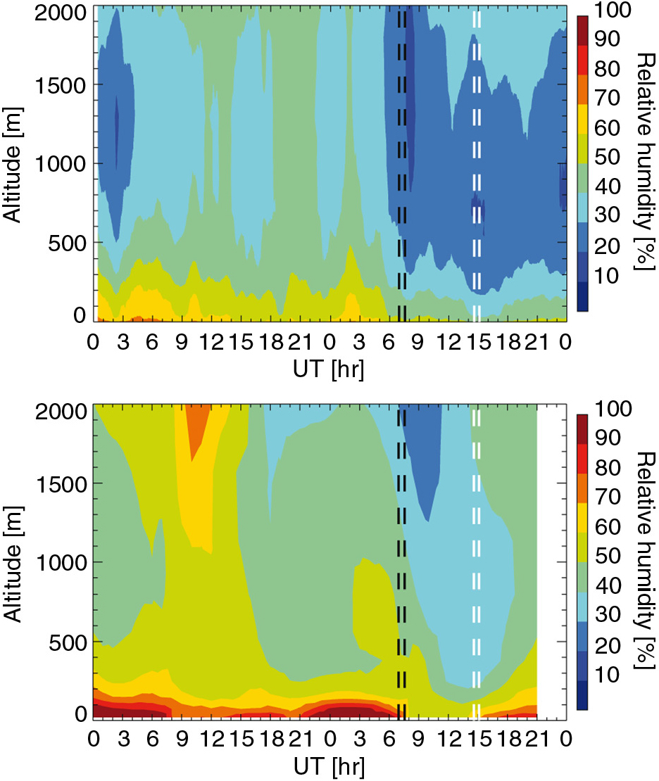
Fig. 4
Time evolution of the relative humidity profiles on 16 and 17 June, as measured by the HATPRO from the ENEA Research Centre (upper panel) and simulated by RAMS at 1 km horizontal resolution (lower panel). The time intervals of the morning and afternoon flights are indicated by black and white vertical dashed lines, respectively.
3.1.1. Simulated meteorological fields and trajectories
Figure 4 compares the time evolution of measured and simulated relative humidity (RH) profiles for the lowest 2000 m of the atmosphere; simulated atmospheric fields at 1 km horizontal resolution are used in the comparison. Although the simulated RH clearly overestimates the measurements, the timing of the dry airmass intrusion and of its arrival at the lowest altitudes, in correspondence with the afternoon flight, are well reproduced.
Figure 5 shows the time evolution of the temperature profile during 16 and 17 June in the lowest 2000 m of the atmosphere, as measured by HATPRO and simulated by RAMS at 1 km horizontal resolution. Although the simulation at 1 km resolution underestimates the surface temperature during the night of 17 June, the overall vertical and temporal behaviour is well reproduced; in particular, the simulation catches the warming occurring below 440 m altitude in correspondence with the afternoon flight (white vertical dashed lines). The altitude of the temperature maximum is shown in Fig. 5 for cases in which a temperature inversion is present: the altitude and timing of the temperature inversions are well reproduced, although with a larger variability in the observations than in the simulations. The inversion is higher on 16 June than on 17 June in both data sets.
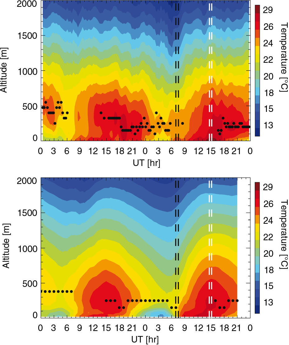
Fig. 5
Time evolution of the temperature profile on 16 and 17 June, as measured by the HATPRO from the ENEA Research Centre (upper panel) and simulated by RAMS at 1 km horizontal resolution (lower panel). Black dots indicate the altitude of the temperature maximum for cases in which a temperature inversion is present. The time intervals of the morning and afternoon flights are indicated with black and white vertical dashed lines, respectively.
The time evolution of the measured wind profile shows a clear diurnal cycle due to the sea–mountain breeze (Fig. 6, upper panel): after sun set (~19–20 UT) the mountain breeze (West-North Westerly flow) replaces the sea breeze (South-South Easterly flow) and persists until sun rise (~7 UT), when the wind starts again to come from the sea. In the 17 June late afternoon, the wind could be retrieved by SODAR up to 200 m altitude. The largest wind intensity was observed at about 250 m altitude between 21 and 24 UT of 16 June. The time evolution of the simulated wind profile is shown in the lower panel of Fig. 6. The daily cycle is well simulated in terms of variability of wind direction, while the wind intensity is generally overestimated; on the other hand, the wind is better represented, also in terms of amplitude, during the night between 16 and 17 June.
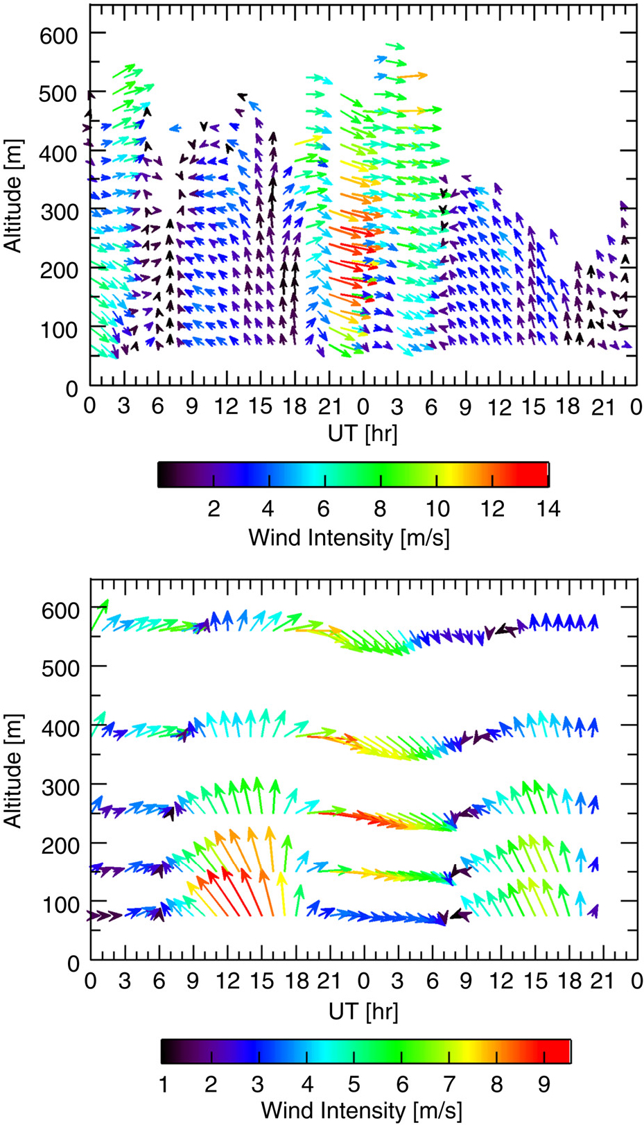
Fig. 6
Time evolution of the measured horizontal wind profile on 16 and 17 June, as measured by SODAR (upper panel) from the ENEA Research Centre and simulated (lower panel) at 1 km horizontal resolution.
Back-trajectories are used to identify the airmass origin. The back-trajectories are calculated with HYSPLIT and M-TraCE using MINNI 3-D fields at 12, 4 and 1 km. Four and a half day HYSPLIT back-trajectories arriving at 7:00 and 15:00 UT, in correspondence with the take-off of the morning and afternoon flights, respectively, are displayed and discussed in the Supplementary file. Both trajectories indicate a progressive descent within ~3.5 d starting at about 4000 m over the Bay of Biscay and following an anti-cyclonic path. Due to the relatively low temporal and spatial resolution of the global NCEP/NCAR reanalysis, the HYSPLIT back-trajectories are not expected to properly simulate the complex interaction between sea breeze and local orography. Figure 7 shows the effect of different 3-D meteorological fields horizontal resolution on the simulated back-trajectories arriving at 100 m (amsl) at 15:00 UT. The time evolution of the HYSPLIT and M-TRACE back-trajectories altitude is also shown. The HYSPLIT back-trajectory arrives from North-West and does not capture the effect of the sea breeze, displaying a slow descent. This is not consistent with the SODAR wind profile (Fig. 6). On the other hand, all the M-TraCE back-trajectories show the ‘trapping’ effect of the sea breeze, which drives the airmass towards the coast from South-East ~2–3 hours after its intrusion in the marine boundary layer. This intrusion occurred ~30 km (~50 km) offshore for the 1 km (12 km) horizontal resolution atmospheric fields. The higher the spatial resolution, the sharper is the rotation and the steeper is the descent of the airmass in the marine boundary layer.
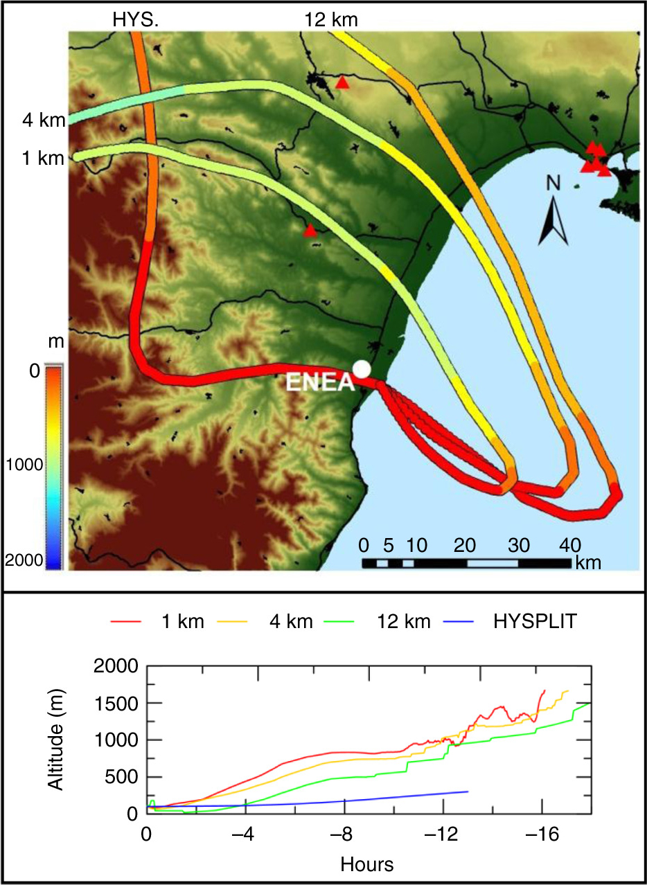
Fig. 7
Upper panel: back-trajectories arriving at the altitude of 100 m during the first afternoon ascent (A1PM) calculated using M-TraCE with 3-D meteorological field at 1 km, 4 km and 12 km horizontal resolution, and using HYSPLIT with NCEP/NCAR global reanalysis. Lower panel: time evolution of the back-trajectories’ altitude.
The influence of the dynamical structure on the aerosol properties in the area of study is described in the following sections through the analysis of the morning and the afternoon airborne measurements.
3.2. Airborne observations: morning flight
3.2.1. Meteorological parameters
The ultralight took off at 6:58 UT (~3.5 hours after sun rise), when the solar zenith angle was 53°. The four vertical profiles of meteorological parameters and aerosol number concentrations are shown in Fig. 8. The profiles were acquired in 35 minutes, within a horizontal distance of 29 km, and provide a detailed view of the atmospheric vertical structure in the study area. The first two profiles were measured within 7.7 km of the airfield, and the last two between 17.5 and 29.1 km of the airfield (Fig. 1b).
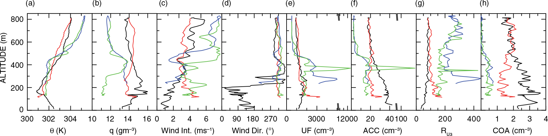
Fig. 8
Vertical profiles of (a) potential temperature, (b) absolute humidity, (c) wind intensity, (d) wind direction, (e) UF, (f) ACC, (g) R U3 and (h) COA during A1AM (black curves), D1AM (red), A2AM (blue) and D2AM (green).
The four vertical profiles show remarkable differences. The morning lower atmosphere was well stratified (Δθ/Δz>0). During A1AM a marked unstable layer (Δθ/Δz= − 5.1 K km−1), which corresponds with the mixed layer, is present in the first 120 m. An abrupt change of q occurs at the top of the mixed layer. The D1AM profile displays a slightly different behaviour of θ, indicating a reduction of atmospheric stability below 350 m, possibly associated with the presence of a residual layer close to the airfield (A1AM). This layer is not observable in the following descent (D1AM). The potential temperature profiles of A2AM and D2AM show significant differences with respect to those of A1AM and D1AM, and display temperature inversions with relative maxima between 500 and 600 m. The values of q measured in the Northern profiles (A2AM and D2AM) were lower than in the Southern ascent and descent (A1AM, D1AM), particularly above 500 m.
Above 250 m altitude, despite the differences in θ and Q, the wind direction was quite homogeneous, with a North-Westerly flow in all profiles. The wind direction was from South-West (i.e. the marine sector) only in the lowest layer of profile A1AM. However, wind intensity displays significant differences in the four profiles. Pronounced wind increases, reaching maxima of ~7 ms−1, occurred in A2AM and D2AM just below the temperature inversions, while large differences between A1AM and D1AM existed below 200 m.
The reader is reminded that the observed differences in the vertical behaviour of wind intensity, θ, and q occur within a horizontal distance of 29 km along the coastline, indicating a significant variability in a limited area.
3.2.2. Aerosol distribution
The vertical distribution of the aerosol concentration is closely linked to the thermodynamic variability and displays very large differences among the four profiles.
3.2.2.1. Coarse particles
High values of COA are observed in profiles A1AM and D1AM, with maxima in the mixed layer during A1AM, where COA reaches values of 3.5 cm−3. Out of the 12 flights of the MORE campaign, the largest values of COA were observed in the afternoon flight of 16 June, with values of ~4 cm−3 in correspondence with the maximum intensity of the Saharan dust outbreak. These are large values of coarse particle concentration associated with a desert dust event for this region. By comparison, Bonasoni et al. (2004) measured hourly COA peak values up to 4.17 cm−3 at the Monte Cimone station (44.2°N, 10.8°E, 2165 m) in the Northern Appenini mountains (~450 km North of ENEA Trisaia).
The reduction of vertical stability observed in D1AM with respect to A1AM and the decrease of COA (and ACC) suggest that a residual layer containing desert dust was present in the ascent (A1AM) close to the airfield. This layer rapidly disappears along the flight towards north. The presence of a relatively large amount of COA particles identified as dust at the lowest altitudes of A1M is consistent with the LIDAR observations (Fig. 3). The A2AM and D2AM profiles display a similar behaviour and very low COA concentration.
3.2.2.2. Accumulation particles
Despite the contribution of desert dust over ENEA, ACC is not very high (up to 40 cm−3, except for a large peak during profile D2AM) as expected for a rural coastal area. Only few studies provide vertical profiles of ACC concentration, which can be compared with our measurements. Analysing the relationship between mixing layer height and balloon-borne measurements of aerosol concentrations over the polluted Po valley in Northern Italy, Ferrero et al. (2010) measured larger values of ACC; they report mean summer values of 35±2 cm−3 and 98±6 cm−3, respectively, above the mixing height and near the surface. The values of ACC measured on the 12 flights at Trisaia were lower than the values by Ferrero et al. (2010), except for the large peak in profile D2AM associated with a thin layer (thickness of ~35 m) with elevated concentration of both UF (~15 500 cm−3) and ACC (~105 cm−3) particles. As discussed in the Supplementary file, these large values of UF and ACC were very likely due to the emissions from a cement plant located about 34 km from the coast.
3.2.2.3. Ultrafine particles
Profiles A1AM and D1AM show quite similar values of UF, while large differences exist in the second ascent–descent.
Measurements of ultrafine particles vertical profiles are very rare in the Mediterranean environment. Mallet et al. (2005) discussed airborne observations of a photochemical pollution event in June in the polluted area of Marseille, Southern France. They measured vertical profiles of particles’ concentration larger than 7 nm, observed ~60 km inland in two consecutive days in the early morning and at noon. On both days, the aerosol concentration in the boundary layer was lower in the morning (~4000 cm−3) than at noon, when it reached values of 12 000 cm−3 in the first day, and more than 40 000 cm−3 in the second day. With the exception of the large peak in the D2AM profile, the noon values shown by Mallet et al. (2005) are much larger than those sampled during MORE.
Two airborne campaigns were carried out at the island of Lampedusa (35.5°N, 12.6°E), in the central Mediterranean, with the same aircraft and instrumentation used in this study. These measurements are relative to an open sea site and can be used as a reference. Six flights were performed during the C-MARE (Central Mediterranean Aerosol and Radiation Experiment) campaign (di Sarra et al., 2005), which took place in the period 20 September–5 October 2004. The overall mean UF profile shows values of ~2500 cm−3 in the marine boundary layer, slowly decreasing to ~1000 cm−3 at 1200 m; a large variability, between 40 and 60% in terms of standard deviation, is associated with the average profile. Six flights were performed between 28 April and 7 May 2008 during the GAMARF (Ground-based and Airborne Measurement of the Aerosol Radiative Forcing) campaign (Meloni et al., 2015). The average UF concentration was ~3000 cm−3 in the first 150 m and decreased to about 1000 cm−3 at 500 m, showing a higher (between 90 and 100%) and lower variability (~30%), respectively, below and above 150 m.
The UF values measured during the four morning profiles discussed in this study are within the range observed during these previous campaigns, except for the cement plant plume sampled in profile D2AM (see Supplementary file for further details).
3.2.3. Descent of dry air with low aerosol content
The region above 500 m in profiles A2AM and D2AM was characterised by very low values of UF, ACC, and COA (about 500 cm−3, 2.5 cm−3 and virtually 0 cm−3, respectively). These low values correspond with minima of q and high values of θ, suggesting a capping of the stable underlying layer, which is characterised by higher values of the aerosol concentration. All these observations indicate the presence of a dry airmass with low aerosol content above 500 m in the Northern part of the flight. As suggested also by the HYSPLIT back-trajectories (Supplementary Fig. 1), by the simultaneous increase in surface pressure (Fig. 2), and by the evolution of temperature, humidity and aerosol profiles (Figs. (3–5)), the dry airmass was descending. The characteristics of the airmasses at the same altitude during A1AM and D1AM were different, with moderate values of ACC and COA (~20 and 1.5–1.8 cm−3, respectively) above 500 m. LIDAR observations also confirm that non-negligible amounts of aerosol were present at the flight altitude in the Southern part of the flight: the backscatter ratio becomes <0.3 only above 1200 m altitude (Fig. 3).
These observations show that the ‘clean’ airmass reached the lower troposphere only in the Northern portion of the flight path, suggesting a strong horizontal variability of the atmospheric dynamical structure within the 30 km spatial scale of the MORE experiment.
High-resolution back-trajectories arriving at 7:00 UT at 100, 350, 600 and 800 m of profiles A1AM and D2AM (respectively the Southernmost and Northernmost profiles) were calculated from the model analyses at 1 km horizontal resolution, and are displayed in Fig. 9. The back-trajectories originate from the Western sector of the domain and display a clear descent. In particular, all trajectories, except part of that ending at 100 m on A1M, follow the orographic structure of the valleys perpendicular to the coast. The dimensions of the 1 km resolution domain (118×130 km) do not allow to study the history of the airmasses at the regional–continental scale, but provide useful indications on the airmasse altitude and origin at the local–regional scale, particularly important for cases of complex orography.
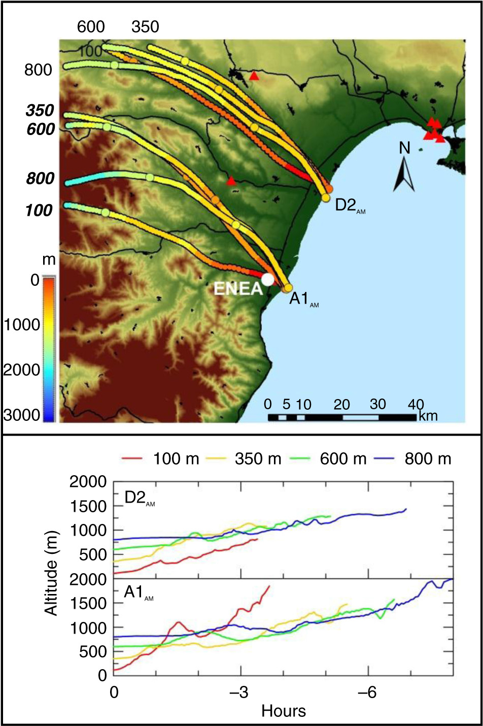
Fig. 9
Upper panel: back-trajectories arriving at 7:00 UT at 100, 350, 600 and 800 m of the A1AM and D2AM profiles. Bold italic characters refer to the A1AM profiles. Three-hour intervals along the trajectories are marked with circles. Lower panel: time evolution of the airmass altitude along the trajectory.
3.3. Airborne observations: afternoon flight
3.3.1. Meteorological parameters
The take-off of the 17 June afternoon flight occurred at 14:40 UT. The four profiles, A1PM, D1PM, A2PM and D2PM, were obtained roughly at the same positions of those of the morning flight. The main measured parameters are shown in Fig. 10. The profiles were acquired in 31 minutes; information on the location and time of each profile is given in Table 2. The prevalent wind for the afternoon flight is from South (marine sector) and is related to the sea breeze daily evolution.
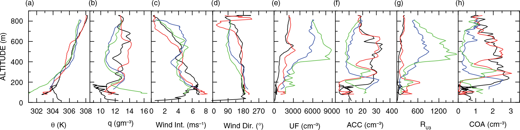
Fig. 10
Vertical profiles of (a) potential temperature, (b) absolute humidity, (c) wind intensity, (d) wind direction, (e) UF, (f) ACC, (g) R U3 and (h) COA during A1PM (black curves), D1PM (red), A2PM (blue) and D2PM (green).
A super-adiabatic temperature profile is observed in the lowest 150 m of A1PM, induced by the land warming and associated with a developed mixed layer (Fig. 10a). At the altitude of 150 m, the aircraft moved over the sea, and an abrupt change from the land to the sea boundary layer appeared. Within less than 400 m of horizontal distance, the values of θ and q changed by 0.5 K and 2 g m−3, respectively, whereas the wind direction remained unchanged. At a distance of 3 km from the airfield, over the sea, the Enduro KIT reached the lowest altitude (~80 m). In that position θ was ~2 K lower than that observed during the take-off (over the land), while wind intensity and q were larger, respectively, by 2 ms−1 and 2.5 g m−3. No significant differences in the wind direction were observed. Thus, the marine boundary layer appeared more stable than the land boundary layer, with a temperature inversion at ~150 m, and higher wind intensity.
The four potential temperature profiles show some similarities, with an almost neutral layer from 400 to 580 m for A1PM and D1PM, and up to 800 m for A2PM and D2PM; both A2PM and D2PM show a temperature inversion at ~350 m, particularly intense in D2PM. The profiles of q are similar in the lowest and highest sections of A1PM and D1PM, whereas differences appear between 400 and 580 m. Between ~300 and 750 m, the values of q for A2PM and D2PM are 15–25% lower than in the first two profiles.
The wind intensity and direction appear similar in all the profiles up to 400 m altitude, while significant differences were observed above this altitude. Southerly winds were dominant, except for the upper portions (above 650 m for A1PM and D1PM, and above 400 m for A2PM and D2PM). As will be shown below, these differences are linked to spatial inhomogeneity in the vertical structure of the sea breeze over the region and indicate that different airmasses are sampled, as suggested by differences in the aerosol concentration.
3.3.2. Aerosol distribution
UF, ACC and COA measured in the mixed layer during A1PM and D1PM display unusually low values, reaching the minima observed in proximity of the surface throughout the MORE campaign. In the lowest 200 m, UF was ~200–300 cm−3, ACC around 5–10 cm−3 and COA between 0.1 and 0.8 cm−3. ACC and COA largely increased above 100–200 m during A1PM and D1PM, while UF showed a somewhat different behaviour, with a gradual increase with altitude. A relative maximum of UF was found around 550 m, just below the temperature inversion separating the (lower) more neutral from the (higher) more stable layers. The aerosol profiles measured during A2PM and D2PM were similar, with large differences with respect to A1PM and D1PM. ACC and COA were largest in the lowest 200–400 m, although significant differences between the two exist. Conversely, UF largely increased with altitude, with a steep transition during D2PM. UF reached maxima of 6300 cm−3 at 650 m in A2PM, and 8900 cm−3 between 400 and 500 m in D2PM. This layer was also characterised by a strong reduction in ACC and COA. The profile of R U3 well highlights the structure of this UF layer, reaching values as large as 1700.
The large differences in the meteorological parameters and in the aerosol concentrations suggest that different airmasses were encountered in the Southern and Northern profiles. Similarly to the morning flight, the descent of relatively dry and clean airmass may be taken as the cause for the behaviour observed in the Northern sector (profiles A2PM and D2PM); this descent apparently continued till afternoon, propagating downwards (down to about 500 m in the morning, and to about 300 m in the afternoon). HYSPLIT large-scale back-trajectories arriving at 17 UT support this interpretation (see Supplementary Fig. 1). Differently from the morning observations, ground-based continuous measurements of aerosol and water vapour vertical profiles at ENEA (Figs. 3 and 4) did not show evidence of a dry airmass with low aerosol content below and above the maximum altitude reached by the aircraft. This is consistent with the aircraft A1PM and D1PM profiles and supports the idea of different airmasses in the Southern and Northern sector of the flight. Although the descending airmasses observed in the Northern sector during the morning and afternoon flight display large similarities (low ACC and COA, low q and high θ) with the morning profiles, the afternoon values of UF were significantly higher.
Figure 11 shows profiles of meteorological parameters, aerosol concentration and Richardson number in the 200–800 m altitude range of A2PM and D2PM. The layer with elevated UF was found in two other profiles (named A3PM and D3PM) acquired inland, whose position along the flight path is highlighted in Fig. 1b by a red oval. Figure 11 also shows the measurements acquired during A3PM and D3PM (respectively orange and purple curves). According to the values of R i, the elevated values of UF occur in a region mostly characterised by turbulent conditions, above the temperature inversions at 350 m. It is possible to estimate a lower limit for the extension of this layer on the basis of the portion of the flight with elevated UF. The layer covers an area of at least 160 km2.
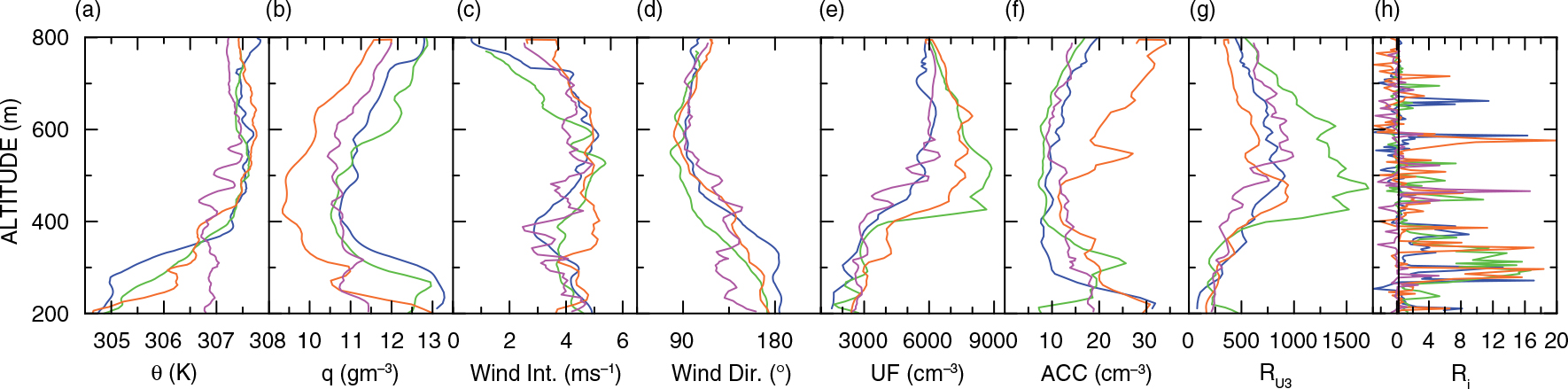
Fig. 11
Vertical profiles of (a) potential temperature, (b) absolute humidity, (c) wind intensity, (d) wind direction, (e) UF, (f) ACC, (g) R U3 and (h) gradient Richardson number during A2PM (blue curves), D2PM (green curves), A3PM (orange curves), D3PM (purple curves). Vertical smoothed profiles of potential temperature and wind intensity and direction used to calculate R i are shown. The value of R i,c is marked by a vertical black line in panel (h).
It is not possible to assess, based on our observations, if this layer was associated with an NPF phenomenon or to the advection of Aitken mode aerosols. However, the elevated UF layer was clearly not connected with an enhanced number of particles in the accumulation mode. Previous studies suggest that NPF events may be triggered by atmospheric mixing processes (Kulmala et al., 2004; Hellmuth, 2006; Lauros et al., 2007, 2011), in some cases due to the break-up of the nocturnal inversion (Stratmann et al., 2003; Wehner et al., 2007; Crippa et al., 2012), to the enhancement of turbulence in elevated layers (Wehner et al., 2010), or to the turbulence associated with the nocturnal low-level jet (Siebert et al., 2007). The occurrence of NPF events has also been linked to the intrusion of descending mid-tropospheric airmasses into the boundary layer (Song et al., 2010), which implies lower values of q than in cases without nucleation (Sogacheva et al., 2007). Both conditions occur also in our case.
Other favourable factors supporting the occurrence of an NPF event (Dunn et al., 2004; Kulmala et al., 2004; Stanier et al., 2004) during A2PM and D2PM are: (1) intense photochemical activity, as suggested by the elevated values of J(O1D) measured during the day (Section 3.1, Fig. 2) and by the high O3 concentration in the layer (not shown), ranging from 70 to 75 ppm, (2) low values of UF observed in the morning, and of ACC in both the morning and afternoon flights, indicating the modest capability of pre-existing aerosol to act as condensation sink for nucleation mode particles or condensable vapours in the descending airmass.
These processes are coherent with our observations and could suggest a possible mechanism favouring NPF events along the coast downwind of the mountain regions. This condition is particularly frequent in the Mediterranean basin.
As discussed in the previous paragraphs, low values of aerosol concentration and absolute humidity are observed in the lowest layers of A1PM and D1PM. This is in agreement with LIDAR and with measurements of q at the surface (Fig. 2). The backscatter ratio profiles also reveal a relative minimum in the aerosol amount in the lowest 100 m during the afternoon flight (Fig. 3).
The M-TraCE back-trajectories arriving at 15:00 UT at 100, 300, 500, and 800 m in correspondence with A1PM and D2PM are shown in Fig. 12. These trajectories, calculated from the 3-D meteorological fields at 1 km horizontal resolution, evidently show the influence of the afternoon sea breeze circulation, and provide an insight into its vertical structure. Striking differences exist with respect to the morning trajectories (Fig. 9); it must be also noted that these morning to afternoon differences, as expected, are not present in the low-resolution HYSPLIT trajectories (Supplementary Fig. 1). Trajectories arriving at 100, 300, and 500 m, and particularly those at 100 m, are advected offshore during the morning, trapped by the sea breeze and subsequently transported towards the coast.
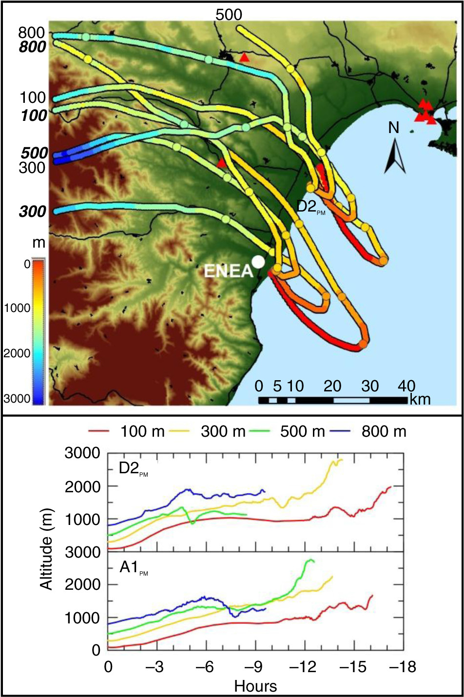
Fig. 12
Upper panel: back-trajectories arriving at 15:00 UT at 100, 300, 500 and 800 m during the A1PM and D2PM profiles. Three-hour intervals along the trajectories are evidenced by larger circles. Bold italic characters refer to the A1PM profiles. Lower panel: time evolution of the airmass altitude along the trajectories.
The back-trajectories can be used to identify also cases of recirculation. For instance, the airmass reaching the A1PM profile at 100 m altitude crossed the path of flight A2AM at ~800 m altitude. Both profiles are characterised by low values of q and very low aerosol amounts. This coincidence provides also a possible explanation for the delay between the minimum value of IWV (~17.5 kg/m2 between 7:30 and 8:30 UT) associated with the overpass of dry airmasses over ENEA, and the minimum value of q at the surface, occurring when the dry airmass is brought inland by the sea breeze.
4. Conclusions
This work presents and discusses the large variability in space and time of the atmospheric thermodynamic structure and the aerosol vertical distribution in a coastal area with complex orography. In situ airborne measurements of meteorological parameters and aerosol concentration, together with ground-based remote sensing observations, were collected in Southern Italy during the MORE campaign that took place in June 2010. These data sets contribute to the MINNI project validation campaign and are used to describe the different processes occurring at the local and regional scales.
The evolution of a specific event occurring on 17 June, when two flights with different vertical profiles were carried out, was studied in details. The measurements were supported by mesoscale model simulations and back-trajectories employing low- and high-resolution (up to 1 hour, and 1 km) meteorological analyses.
The event was characterised by the arrival of a dry and nearly aerosol-free descending airmass, which interrupted a Saharan dust event. Although some indications suggest that an NPF phenomenon might have occurred in the descending airmass, additional measurements of ultrafine particles would be needed to address this type of process. The local circulation was also strongly affected by the daily evolution of the sea breeze, leading to recirculation of the airmasses; also local pollution plumes were found in the air sampled.
Vertical profiles of the thermodynamic variables and the aerosol distribution display a large variability within the region of the aircraft measurements, influenced by long-range transport, regional scale and local dynamical processes.
The high-resolution simulations carried out with RAMS are capable of reproducing most of the observed features, including the sea breeze regime. The trajectory analysis clearly shows that high-resolution meteorological fields are necessary to interpret the observations in such a complex environment.
The measurement strategy must specifically address the high spatial and temporal variabilities which are typical of this context. This study shows that the information on the vertical profiles is crucial for the understanding of the occurring processes, and the synergy among ground-based remote sensing continuous measurements, in situ airborne observations and high-resolution regional modelling is essential to understand the interactions of processes acting on different scales. In particular, the opportunity to perform repeated flights as well as the timing and location of the vertical profiles are essential to capture key aspects of the diurnal cycle and the connections between local and large-scale phenomena.
The investigation of new particles nucleation formation phenomena may benefit from the approach used in this study, although specific measurements of ultrafine particles are essential for the understanding of these processes. This type of measurements is generally available on the Enduro KIT ultralight aircraft, but was not operational during MORE.
A limitation faced during the airborne campaign was the confinement to the maximum flight altitude due to the Italian legislation in force at that time. This restriction prevented observations into the free troposphere, which might have helped to address regional-scale meteorological and aerosol regimes. The results of this campaign confirm the usefulness of airborne in situ measurements within the planetary boundary layer for testing air quality models.
Acknowledgements
This work has been carried out with the support of the EUFAR Transnational Access, and the data used to produce these results are available upon request to the corresponding author. This work has been supported by the Italian Ministry for Environment and Territory and Sea through the MINNI (Integrated National Model in support to the International Negotiation on Air Pollution) project and partly by the Italian Ministry of Education, University and Research through Projects NextData and RITMARE. We especially thank G. Casasanta, L. De Silvestri, C. Di Biagio, N. Di Genova, S. Finardi, D. Mateos, I. Mavilia and G. Tomei for their active contribution to the MORE project. Helpful comments and suggestions by two anonymous reviewers and the editor are also acknowledged.