
1. Introduction
The major sink of atmospheric molecular hydrogen, H2, is the uptake by soil. This uptake totals about 60 Tg H2/yr and is a widespread process: Virtually, all soils containing organic carbon were shown to take up H2. Moreover, the uptake was shown to be predominantly biological – mediated by enzymes, i.e. by various kinds of hydrogenase (see Conrad, 1999; Constant et al., 2010), and to take place in the uppermost 10 cm of the soil (Liebl and Seiler, 1976; Förstel, 1986; Yonemura et al., 1999).
The rate of uptake is usually expressed as deposition velocity, vd [cm/s], such that the flux of H2 from the atmosphere to the soil surface, Fa [molec/cm3/s], is given by
where ρ is the number density of air molecules in [cm−3], and Ma is the volume mixing ratio of H2 at the soil surface.
This deposition velocity was measured by numerous in situ experiments for various biomes and shown to vary between 0.01 and 0.1 [cm/s] (see Ehhalt and Rohrer, 2009, for a summary). The field measurements also demonstrated a significant decrease of vd with increasing soil moisture except occasional observations of very low vd for very dry soils. The temperature dependence of vd measured in the field was relatively weak and exhibited a broad maximum around 30°C (Liebl and Seiler, 1976; Conrad and Seiler, 1985; Förstel, 1986; Yonemura et al., 1999; Yonemura et al., 2000a, 2000b; Lallo et al., 2008; Schmitt et al., 2009). Unfortunately, the measurements so far do not suffice to characterize all relevant types of soil, and the estimates of global average uptake based on them involve large extrapolations.
More recently, there have also been several attempts to formulate theoretical expressions for vd (or of Fa directly), which allow us to predict its dependence on soil moisture and temperature (Yonemura et al., 2000b; Smith-Downey et al., 2008; Schmitt et al., 2009; Bousquet et al., 2011). They were based on 1D molecular diffusion of H2 into and within the soil and on its enzymatic removal within. To achieve simple expressions, it was usually assumed that the soil parameters (soil porosity, moisture, temperature, as well as enzymatic activity) are uniform throughout the soil. Thus, most of these studies disregarded the observation that the top layer of the soil is often so dry that its enzymatic activity is greatly diminished or even totally destroyed (Yonemura et al., 2000b; Smith-Downey et al., 2008). Recognizing this, Yonemura et al. (2000b) therefore proposed a two-layer soil diffusion model for the uptake of H2. The upper layer is assumed to be devoid of hydrogenase activity and acts essentially as a diffusion barrier. Its thickness, δ, on the order of 1 cm, increases with dryness. In the layer below, both diffusion and removal of H2 take place. The authors solved the model numerically, and the results matched reasonably well the observed dependence of vd on soil moisture.
Here we will show that using this model and virtually the same assumptions about soil uniformity as Yonemura et al. (2000b), we can obtain an analytical solution for vd (Section 2). This solution explicitly depends on δ.
To characterize the enzymatic removal rate of H2 within the soil and its dependence on soil moisture and temperature, we rely on published data from laboratory experiments (Section 3). With an expression for the average dependence of δ on soil moisture, which is derived in Section 4, we can formulate a complete dependence of vd on soil moisture and temperature. In Section 5, the vd calculated from our analytical expression is compared against those disregarding the effects of a dry layer and a set of vd from field measurements. The implications are discussed.
2. Derivation of a closed expression for vd
2.1. Diffusion equations
Following the earlier studies (Yonemura et al., 2000b; Smith-Downey et al., 2008), we assume that molecular diffusion drives the transport of H2 within the soil. We further assume that there is no production of H2 in the soil and that the destruction is first order in the H2 concentration. Therefore, the 1D diffusion equations for flux and mass balance take the form:
where Fs is the flux in molec cm−2 s−1, ρ is the number density of soil air in molec cm−3, Ms is the mixing ratio of H2 in soil air, and z is the depth in cm. ks is the rate constant for removal of H2 from soil air in s−1. ks −1=τ, the mean lifetime of H2 in soil air.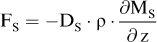

Θa is the fraction of soil volume filled with air. It is given by
where Θp is the total porosity of the soil (cm3 total pore space/cm3 soil), and Θw is the volumetric soil water content (cm3 of water-filled pores/cm3 soil).
DS is the diffusivity of H2 in the soil (units: cm2 s−1). There are several ways to formulate DS. Following Millington and Quirk (1961) (see also Yonemura et al., 2000b; Schmitt et al., 2009), DS can be expressed as:
where DA is the molecular diffusivity of H2 in air (units: cm2 s−1). DA depends on temperature, T in °C, and atmospheric pressure, p in hPa (see Yonemura et al., 2000b):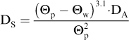

Our calculations will assume steady state, i.e.

2.2. Two-layer model
To calculate the deposition velocity, we apply these diffusion equations to a two-layer soil model first proposed by Yonemura et al., 2000b. It consists of an upper dry layer (I) of depth δ without H2 removal and a more moist layer (II) below, in which H2 is destroyed enzymatically at a rate characterized by the uniform rate constant ks. Since layers I and II differ in soil moisture, Θw, they also differ in diffusivity, DS [see eq. (5)]. The deposition velocity is defined by eq. (1) given above to
In layer l the hydrogen flux, FI, remains constant and equal to Fa. In that layer, i.e. for 0≤z≤δ, the gradient in Ms is therefore linear and given bywhere Ms(0)=Ma and Ms(δ) are the H2 mixing ratios in the soil at depths z=0, and z=δ, respectively.

For z≥δ, i.e. layer II, the vertical profile of Ms is determined by eq. (7). Assuming DSII, ρ, Θa, ks to be constant with depth, eq. (7) can be solved analytically:
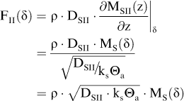
The H2 flux at depth δ can be calculated by inserting solution (10) in eq. (2) Or solving for Ms(δ)Inserting eqs. (12) and (8) into eq. (9), and observing that Fa=FI=FII(δ), and Ma=Ms(0), we solve for vd and obtainEq. (13) presents an analytical expression for vd. Besides the simple soil parameters, DSI, DSII, Θa, it also contains the more involved quantities δ and ks. The latter also depend on the soil moisture; ks also on the soil temperature. Thus, before eq. (13) can be used to describe the dependence of vd on soil moisture and temperature, expressions for those individual dependencies must be found. This will be done in the two following sections.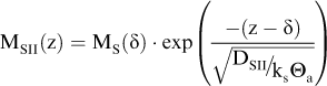
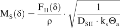
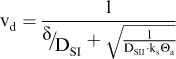
In passing, we note that eq. (13) unifies two special cases that have been used earlier to parameterise vd. For moist soils, δ approaches 0, and eq. (13) reduces to the solution as derived by Yonemura et al. (2000b) for their one-layer model (see also Smith-Downey et al., 2008). For very large δ, i.e. , eq. (13) reduces to Vd=DSI/δ, the expression used by Schmitt et al. (2009).
3. The dependence of ksΘa on soil temperature and soil moisture
ks and its dependence on soil moisture and temperature can and has been determined by laboratory experiments. To be exact, what these experiments have determined is the functional form of the dependence of ksΘa on temperature and moisture (see Ehhalt and Rohrer, 2011). Moreover, as the experiments of Smith-Downey et al. (2006) demonstrated, the dependences on soil moisture and temperature can be separated, i.e., ksΘa can be written as
where A is an adjustment factor to account for different amounts of hydrogenase in the soil under investigation, f(Θw) characterizes the soil moisture dependence, g(T) the dependence on soil temperature. As it turns out, g(T) is virtually identical for all soils investigated so far – at least for temperatures<40°C. f(Θw), however, appears to differ between different soils (Conrad and Seiler, 1981; Ehhalt and Rohrer, 2011). For both of the functions, f(Θw) and g(T), we rely on the reanalysis by Ehhalt and Rohrer (2011) of previous laboratory data. They obtained the following for the temperature dependence:
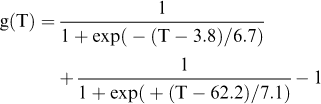
For the moisture dependence fes(Θw/Θp) of eolian sand and fll(Θw/ Θp) for loess loam they found
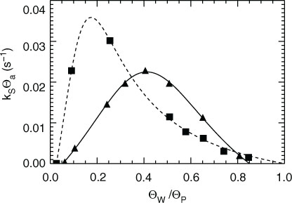
The latter functions were derived for Θw/Θp as moisture variable rather than Θw for better comparison with other experiments. They hold for 0.0264≤Θw/Θp≤1 and 0.0537≤Θw/Θp≤0.851, respectively, and are zero elsewhere. The lower bounds are caused by the threshold moisture below which the enzymatic uptake of H2 vanishes; the upper bounds are caused by the disappearance of air-filled pores. Eqs. (16) and (17) are based on the measurements by Conrad and Seiler (1981).

The only other soil for which f(Θw/Θp) has been published is boreal forest soil (Smith-Downey et al., 2006), which has also been reanalysed by Ehhalt and Rohrer (2011). The function g(T) is depicted in Fig. 1; the functions fes(Θw/Θp) and fll(Θw/Θp) are shown in Fig. 2. For more details, see Ehhalt and Rohrer (2011).
Fig. 1.
Removal rate constant of H2 in soil as a function of temperature, eq. (15) (after Ehhalt and Rohrer, 2011). The decreasing branch of the profile, dashed line, is less well defined and may depend on the actual soil type and region.
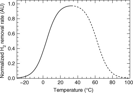
Fig. 2.
Removal rate constant of H2 in soil, ksΘa, as a function of soil water saturation, Θw/Θp. Squares represent eolian sand and triangles represent loess loam, eqs. (16) and (17) (after Ehhalt and Rohrer, 2011).
4. The dependence of δ on soil moisture
The depth δ is an auxiliary quantity. It captures with a single parameter the essence of the influence of the vertical soil moisture profile on vd. This simple parameterisation seems justified, since well-resolved vertical profiles of soil moisture are hardly ever reported when vd is measured. Under the best circumstances, the average soil moisture across the top 10 cm of soil is available – usually measured by time domain reflectometry. Thus, to enable comparison with field experiments, we choose this average, , as a measure of soil moisture.
To derive an expression for the dependence of δ on , we proceed semi-empirically. We first calculate sequences of realistic soil moisture profiles with the help of the 1D model of HYDRUS.1 [1] The calculations assume a 4 m deep uniform soil column with a total porosity, Θp=0.38, and temperature, T=15°C, bounded at the lower end by the water table. The vertical resolution dh varies from 0.008 cm at the upper bound to 0.8 cm at the lower bound according to (dh)2=h/625 cm−1+0.0082 cm2. For realistic upper boundary conditions, we select the measured daily mean values of rainfall, air temperature, and relative humidity obtained at the weather station of the Jülich Research Centre during the year 2008. Two types of soil are investigated: Sandy loam, and loam. For technical reasons, the profiles are read out every 1.5 days.
From eq. (14) and the calculated soil moisture profiles, we generate vertical profiles of the removal rate, ksΘa, from which we will eventually estimate δ.
To illustrate the types of profiles obtained, Fig. 3 describes the sequences of profiles of soil moisture and removal rate in sandy loam and loam during a dry spell of about two weeks following a day with rainfall (27 April 2008). As the sequence for sandy loam indicates, the soil moisture profile develops a shallow dry layer with ΘW close to zero and about 0.1 cm depth within 1.5 days. With increasing time, this layer deepens and reaches about 1 cm depth after two weeks. The dry layer maintains a finite level of soil moisture which depends somewhat on the model assumptions. The exact value of that moisture is, however, not important, as long as it remains lower than the threshold moisture below which the enzymatic H2 uptake vanishes. This dry layer is bounded below by a narrow zone of rapidly increasing moisture followed by a more gradual increase in moisture at greater depth. The zone of rapid increase in soil moisture has been termed ‘evaporation front’ or ‘drying front’ to stress the fact that soil water transport proceeds in the form of water vapour above and in the form of liquid water below the front (e.g. Saravanapavan and Salvucci, 2000).
Fig. 3.
Vertical profiles of the volumetric soil water content, Θw, for (a) sandy loam and (c) loam calculated using HYDRUS. The corresponding vertical profiles of the hydrogen removal rate in soil, ksΘa, calculated from these moisture profiles using eq. (16) or (17) for ksΘa(ΘW) are shown in the right panels (b, d). The profiles were calculated for a dry spell lasting about 2 weeks at 0, 1.5, 3, 6, and 12 days after the last rainfall.
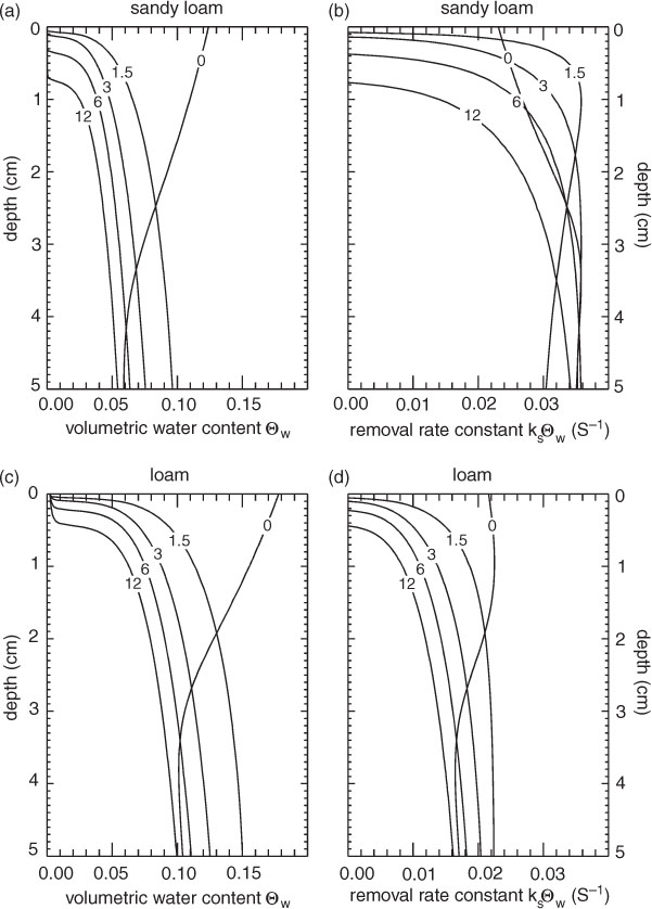
The corresponding profiles of the removal rate constant, ksΘa, are similar to those for soil moisture. For sandy loam, the rapid increase is even accentuated owing to the fact that the dependence of ksΘa on Θw for sand, eq. (16) shows a steep rise at low Θw (see Fig. 2). As a consequence δ is quite well characterized. In the following, δ will be defined as the depth at which the ½ – value of the maximum ksΘa in the top 10 cm of soil is reached. Panel (3a) also indicates that ksΘa in a given profile is fairly uniform at greater depths. Hence, it corroborates the two-layer model which approximates the actual ksΘa profiles by a Heaviside function with a jump of ksΘa from 0 to a finite, constant value at depth δ.
A similar picture emerges for loam – except that the soil remains moister and the dry zone shallower (Fig. 3b). In addition, the depth profiles for ksΘa are more gradual owing to the slower increase of ksΘa with soil moisture for loam, eq. (17).
The δ so obtained from the various annual series of profiles are plotted against the corresponding in Fig. 4, where is obtained from integrating the soil moisture profiles over the first 10 cm. The total ensemble of data points follows similar hyperbolical curves. However, Fig. 4 also indicates that the individual soils actually have their own hyperbolical shapes with the curves for the soils of smaller pore size ranging over higher average soil moistures, . The full curves represent least square fits to the data for sandy loam, eq. (18), and loam, eq. (19):
They hold for 0.02≤≤Θp in the case of δs, and for 0.03 ≤≤Θp in the case of δL.

Fig. 4.
The dependence of δ on the average volumetric soil water content, , calculated for various soils (blue diamonds: sandy loam; red crosses: loam). The full curves represent fits to the data for sandy loam, and for loam, respectively.
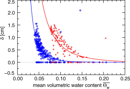
Eq. (18) should hold for all sandy soils. In fact, we also calculated δ for pure sand, but the data clustered too closely for a meaningful fit. Nevertheless, they were compatible with eq. (18). Moreover, calculations for loamy sand were reasonably close to that for sandy loam.
In the choice of the functions and their argument, (Θp – )/, we were guided by the observations that: (1) δ=0 when all the soil pores are filled with water, i.e. when =Θp; (2) δ approaches 10 cm when approaches the level , the soil moisture where the H2 removal rate vanishes; (3) δ() is monotonic. The latter suggests a power function or a power series for δ(). For simplicity we choose a power function. Obviously, the derived δ() depends on the choice of Θp and ks(T, Θw) Θa, but mostly it depends on the type of soil chosen in modelling the depth profile of ΘW.
We also note that the actual data points scatter substantially around the average curves for δS() and δL(). The reason is, of course, that different profiles of soil moisture – leading to different δ - can result in the same . In particular, δ-values of zero are reached even at the lowest . This occurs when soil moisture profiles are sampled during the time of rainfall. Then the soil moisture exceeds even in the topmost soil layer. Therefore, δ depends not only on but also on the immediate history of rainfall and evaporation. It also means that the use of eqs. (18) and (19) will introduce an additional uncertainty in the eventual calculation of .
5. Discussion
With the help of eq. (14) for ksΘa, and eq. (18) or eq. (19) for δ, we can calculate vd from eq. (13) for sandy or loamy soils, if Θp, and T are known. In particular, we can calculate the dependence of vd on for such soils. Figure 5 presents examples for sandy soil and loam, and compares them with the corresponding vds from the single-layer model, where . For the later comparison with field measurements of vd, the shown dependences are based on Θp=0.38, T=15°C. Moreover, the calculations assume eq. (16) for the moisture dependence of ksΘa in sand and eq. (17) for that in loam. For both soils, the parameter A in eq. (14) was set to 1, and the soil water contents ΘWI in the top layer δ to , where is the threshold moisture below which ksΘa vanishes. For Θp=0.38, it is 0.01 for sandy soil, and 0.02 for loam. ΘWII is then calculated by placing the remaining, major fraction of in the soil layer between δ and 10 cm:
Eq. (20) holds for δ≤5 cm.
Fig. 5.
Deposition velocity, vd, as a function of the average volumetric soil water content, (heavy full line: loess loam two-layer model; thin full line: loess loam single-layer model; heavy dashed line: sandy soil two-layer model; thin dashed line: sandy soil single-layer model).
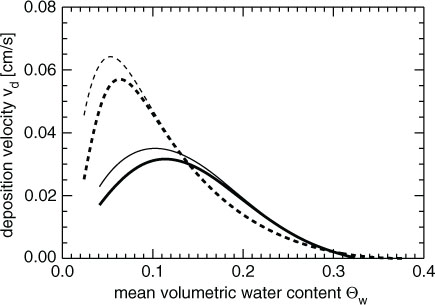
Figure 5 demonstrates three major features in the dependence of vd on . (1) All profiles exhibit the same general pattern, namely vd=0 for , vd approaching 0 when approaches Θp, and a more or less broad maximum in between. (2) The form of vd() differs significantly for different soils. This is caused mainly by the difference in ksΘa(Θw). (3) The inclusion of a dry top layer introduces a significant decrease in the calculated vd at smaller . That decrease can amount to up to 40% and depends on the type of soil.
The validity of vd predicted from eq. (13) can be tested: (1) By comparison with existing field measurements of vd in soils, for which , Θp, and T have also been measured. (2) By comparison with the numerical results from modelling an idealized soil. In the second case not only Θp and T can be specified, but also vertical profiles of Θw and ksΘa in the soil, providing a much more detailed characterization of the soil conditions. In fact, with such information vd can be calculated directly by numerically solving the differential eq. (7). With the data on vertical profiles of Θw and ksΘa acquired for deriving δ in Section 4 we can exactly do that. Figure 6 shows the results for sandy loam and loam. The full curves are the two-layer model cases from Fig. 5 and represent the average dependence of vd on . They agree well with the data points calculated numerically from the individual profiles of Θw and ksΘa. The agreement with the one-layer model is significantly less. This test clearly favours the two-layer model.
Fig. 6.
Dependence of vd on for (a) sandy loam and (b) loam. The full squares represent the numerically calculated values of vd for individual profiles of Θw and ksΘa; the full lines represents the average vd() based on eq. (13) for vd and eqs. (18) and (19) for δ. The thin lines indicate the average vd() from the corresponding one-layer model.
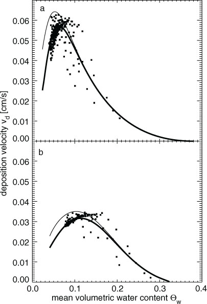
However, we note that even in that case, the individual data points can deviate substantially from the mean, a fact that was already observed for δ (Fig. 4) and assigned to the observation that quite different profiles of Θw can lead to the same . We further note that for vd the deviations tend to become larger for larger . A likely explanation is that longer periods without rainfall are required to generate dry soils. During that time the moisture profiles reach similar and regular shapes (see Fig. 3). In contrast, during periods of frequent rainfall events and therefore higher water content, the moisture profiles maintain more irregular and varied shapes.
The deviations of the individual vd from the mean predicted by eq. (13) (Fig. 6) can be used to estimate the possible fluctuations of individual vd measured in the field caused by variability that is unaccounted for in the moisture profiles. The relative deviations for loam, δvd, show an average moisture dependence well approximated by the relation:
The comparison with field data is hampered by the lack of vd measurements that are accompanied by measurements of the three parameters, Θp, Θw, and T needed to apply eq. (13). We were able to find only one such set of measurements, namely that by Schmitt et al. (2009). These measurements were made over bare loess loam at four different sites spaced about 30 m apart, and in monthly intervals from January to December 2007. The total porosity, Θp, averaged 0.38. The temperature given was measured inside each sampling enclosure and averaged 15°C, but ranged from 0°C to 35°C. The soil moisture averaged over the upper 10 cm was measured at each site by time domain reflectrometry. The measured vd and their dependence on are summarized in Fig. 7.
Fig. 7.
Deposition velocity, vd, as a function of the average volumetric water content, , for loess loam. The triangles mark the vd measured by Schmitt et al. (2009) – the open triangles referring to site 1. For clarity, only one pair of the experimental errors is given. The error in is the same for all data points. The error in vd varies, but is in most cases the size of the symbols. The heavy full line represents vd calculated from eq. (13) for T=15°C using eq. (19) for δ and eq. (17) for ksΘa with a scaling factor A=2. The upper and lower bound of the dark shaded area indicate the corresponding vd calculated for 30°C and 0°C, respectively. The uncertainty introduced by the use of eq. (19) for δ is indicated by the superimposed light shaded area. The thin curve represents a vd calculated from eq. (13) with A=8 and T=30°C.
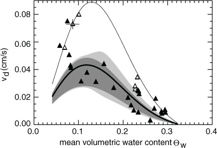
Clearly, the vd measured in the field reach values more than a factor of two higher than those calculated for loam in Fig. 6b. This indicates that the uptake rate constant, ks(Θw,T)Θa, in the bare loess loam was higher than that assumed in Fig. 6b, and suggests that the scaling factor A in eq. (14) must be significantly larger than 1 to fit the measured data. We further note that the scatter in the experimental vd appears even larger than that observed in Fig. 6b. One explanation is that ks(Θw,T)Θa varied with time. This is most likely because the temperature varied with season. A second possibility is that the enzymatic activity varied from site to site. This possibility is also quite plausible considering that the vd from site 1 — indicated by the open triangles in Fig. 7 – all tend to fall into the upper range of the measured vd().
To accommodate the latter possibility, we present two choices of vd() calculated from eq. (13): One with A=2, the other with A=8. The heavy line assumes A=2, eqs. (14), (15), and (17) to characterize ksΘa(,T), eq. (19) for δ, Θp=0.38, and T=15°C. To provide a sense of the spread in vd introduced by the range in observed temperatures or by the variance of the soil moisture profiles leading to the same , it is accompanied by error bounds. The dark area gives the range of vd due to the range in T. It is obtained by calculating vd from eq. (13) for T=0°C and 30°C, respectively, but otherwise the conditions are identical. (The relatively small spread with temperature apparent in the calculated vd also offers an explanation why the vd observed in the field show a large dependence on Θw but a weak one on T.) The light shaded area covers the deviations due to the variance in the soil moisture profiles. It is obtained by multiplying vd() for 30°C with () from eq. (21) and by dividing vd() for 0°C by that term.
The thin line makes the same assumptions as that for A=2, except that A=8 and T=30°C; the latter to account for the fact that the largest vd was obtained at temperatures≥30°C.
Obviously, the comparison of the modelled vd() with this set of field data is not conclusive. On the one hand, the upper and lower most of the measured vd appear to follow envelopes which are compatible with the modelled dependence of vd on . In particular, vd() for A=2, and its error bounds cover the field data – apart from those from site 1 – reasonably well. This is gratifying, since apart from the factor A, the calculated vd() is not based on the field data for vd, but are derived from independent information: Laboratory measurements for ks(Θw,T)Θa and model calculations for δ.
On the other hand, the field data on vd as a whole do not show the moisture dependence predicted by eq. (13). In fact, their dependence is most accurately fitted by a straight line. For the data without those from site 1, the regression line takes the form vd=0.065 – 0.2*, with a standard deviation of 0,009 cm/s. For comparison, the standard deviation of these data from the vd() predicted from eq. (13) with A=2 is 0.013—clearly a worse fit.
There are several reasons for this: (1) The present field data do not reach to low enough to produce an unequivocal turnaround in the measured vd. (2) The data are not homogeneous enough. They are possibly influenced by a variation in ks(Θw,T)Θa from site to site, which makes it impossible to describe them with one single factor A or a single temperature. (3) They are not numerous enough to select sufficiently large subsets of vd measured at the same site and at the same temperature and thus to remove some of the variance in the vd. (4) Eq. (17) for ksΘa() used to model vd might not exactly match the ksΘa() acting in the measured soils. Indeed a superposition of eqs. (16) and (17) corresponding to a small admixture of sand would shift the maximum in the resulting ksΘa() to lower and yield a better fit of vd() from eq. (13) to the field data.
For reasons 1–3, these field data also do not lend themselves to differentiate between the vd() predicted from a one-layer and a two-layer model.
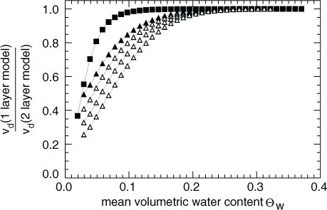
The differences between vd() from a one-layer and a two-layer model vary not only with the type of soil (Fig. 6), but also with the enzymatic activity in the same type of soil. The latter is demonstrated in Fig. 8 which compares the ratios of vd(two layer) to vd(one layer) as a function of for loam with various values of A. This ratio deviates significantly and increasingly from 1 for <0.15 and A>1. Such moistures are quite common even at relatively humid mid-latitudes. From the fact that the vd measured in the field can reach 0.1 cm/s (see Ehhalt and Rohrer, 2009), we can also conclude that A>1 in most natural soils and often reaches up to 8. That means for many field conditions we must expect the actual vd to be smaller than that calculated from a one-layer model. At the same time, Fig. 8 indicates that there is no single correction formula to convert vd from the one-layer model to a vd calculated with the two-layer model. We, therefore, recommend the use of eq. (13) for calculating vd, although it means a slightly larger calculation effort. This should lead to a significant improvement in the calculated vd especially in dry climates.
Fig. 8.
Ratio of vd from the two layer to that of the one-layer model as a function of . Full squares represent sandy soil for A=1. Full triangles represent loam for A=1; open triangles are for loam with A=2, 4, and 8.
In fact, a general application of process-based calculations of vd – whether based on a one-layer or two-layer model – is hampered far more by the lack of data on ks(Θw,T)Θa. That moisture dependence has been determined only for three soils: In addition to the two soils described here, sand and loess loam, ks(Θw,T)Θa has been determined for boreal forest soil by Smith-Downey et al. (2006). This limits a global calculation of soil uptake with the help of eq. (13). On the other hand, many soils consist of a mixture of loam and sand as the major components. Thus, appropriate interpolations between eqs. (16) and (17) for ks(Θw,T)Θa and between eqs. (18) and (19) for δ could be used to treat those cases until measurements of ks(Θw,T)Θa in further soils become available.
6. Summary and conclusions
We derived an analytical expression for the deposition velocity of H2 on soil, vd, which explicitly describes the dependency of vd on the average soil moisture, , and temperature, T, of the soil, which are the only dependencies that have been identified so far. The derivation is based on a two-layer soil model originally proposed by Yonemura et al. (2000b). It consists of a dry top layer with a depth, δ, free of H2 removal and a moist deeper layer with a uniform H2 removal rate constant, ksΘa. With a few further assumptions – notably uniform moisture and therefore uniform diffusivity, DS, in each of the layers – we solve the 1D vertical diffusion equation in each layer. By matching the H2 fluxes at the boundaries, we obtain three equations which can be solved for vd in terms of δ, DS, ksΘa. For a quantitative estimate of vd an approximate expression for δ() is derived. As it turns out δ is not a unique function of , but influenced by other factors such as the immediate history of rainfall and evaporation. The derived vd shows a relatively weak dependence on T, but varies strongly with . The dependence on exhibits a broad maximum of vd around =0.12 for loess loam and =0.07 for sandy soil. vd approaches 0 as approaches 0.38, the value of ΘP. The decrease of vd to low is steep and reaches 0 at a threshold ~ 0.02 or 0.01, respectively. A comparison of the calculated vd() with field measurements is hampered by the lack of suitable data. For >0.05, where field data on vd exist, the agreement is reasonable. A comparison with numerically calculated vd() from a completely characterized artificial model soil gives good agreement and favours the vd calculated from the two-layer model over that calculated from a one-layer model.
7. Acknowledgement
We would like to thank Dr. Michael Herbst for the introduction to and help with the HYDRUS model.