
1. Introduction
It is well known that four-dimensional variational data assimilation (4DVar) (e.g. Lewis and Derber, 1985; Le Dimet and Talagrand, 1986; Courtier and Talagrand, 1987; Courtier et al., 1994; Bormann and Thepaut, 2004; Park and Zou, 2004; Caya et al., 2005; Bauer et al., 2006; Rosmond and Xu, 2006; Gauthier et al., 2007) has provided a useful and robust tool for numerical weather prediction (NWP), especially as more and more observation data becomes available via remote sensing techniques. 4DVar has the following two attractive features: (1) the physical model provides a temporal smoothness constraint; (2) it can simultaneously assimilate the observations at multiple time points in an assimilation window. Generally speaking, the successful use of the incremental method (Courtier et al., 1994) and adjoint technique (e.g. Lewis and Derber, 1985; Le Dimet and Talagrand, 1986; Courtier and Talagrand, 1987) has opened a new era in the numerical weather forecast and they are widely used at many operational numerical weather forecast centres (e.g. Bormann and Thepaut, 2004; Park and Zou, 2004; Caya et al., 2005; Bauer et al., 2006; Rosmond and Xu, 2006; Gauthier et al., 2007). Unfortunately, due to its strong dependence on the adjoint model of the forecast model (Bormann and Thepaut, 2004; Park and Zou, 2004; Caya et al., 2005; Bauer et al., 2006; Rosmond and Xu, 2006; Gauthier et al., 2007), computer implementation of 4DVar is often expensive and not easy to program because of the need to maintain and update the adjoint model of the forecast model. The situation is even worse when the forecast model is highly non-linear and/or the model physics involves discontinuous parameters (Xu, 1996). Furthermore, the applications of the static, thus flow-independent, background-error covariance in the traditional 4DVar often causes its poor assimilation performance (Beck and Ehrendorfer, 2005; Zhang et al., 2009; Cheng et al., 2010).
On the contrary, ensemble Kalman filter (EnKF; cf. Evensen, 1994, 2004; Houtekamer and Mitchell, 1998; Keppenne, 2000; Anderson, 2001; Houtekamer and Mitchell, 2001; Whitaker and Hamill, 2002; Ott et al., 2004; Zhang et al., 2004; Hunt et al., 2007) provides another advanced method for data assimilation. EnKF becomes increasingly attractive due to its simple conceptual formulation and relative ease of implementation. Moreover, it has the capability to provide flow-dependent error estimates from the statistics of the ensemble samples. However, unlike 4DVar, EnKF cannot guarantee the dynamic balance in its results since it is essentially a sequential data assimilation method.
The foregoing analysis shows that in order to maximise their full potential 4DVar and EnKF should be coupled to form a more efficient composite method, which seems a natural idea to compensate the shortcomings of both methods by combining their strength (e.g. Lorenc, 2003; Harlim and Hunt, 2007; Tian et al., 2008, 2011; Wang et al., 2010; Zhang et al., 2009; Cheng et al., 2010; Zhang and Zhang, 2012; Wang et al., 2013). According to the classification suggested by Andrew C. Lorenc (http://www.wcrp-climate.org/WGNE/BlueBook/2013/individual-articles/01_Lorenc_Andrew_EnVar_nomenclature.pdf), the existing composite methods in the literature can be roughly divided into three groups, namely, the ‘hybrid’ (e.g. Wang et al., 2008a, 2008b; Clayton et al., 2013), the ‘En4DVar’ (e.g. Zhang et al., 2009; Zhang and Zhang, 2012) and the ‘4DEnVar’ assimilation methods (Qiu et al., 2007; Liu et al., 2008; Tian et al., 2008; Wang et al., 2010; Tian et al., 2011; Tian and Xie, 2012). The ‘hybrid 4DVar’ denotes 4DVar methods using a combination of climatological and ensemble covariances. In the ‘En4DVar’, the EnKF and 4DVar runs are implemented in parallel and the information is exchanged complementarily (Zhang and Zhang, 2012): The resulted data assimilation system is based on an ensemble forecasting framework in which EnKF is used to estimate the ensemble background covariance and to update the analysis perturbations, while the 4DVar analysis is performed afterward and is taken as the final analysis for the combined 4DVar and EnKF method. Here 4DVar is implemented in its traditional way except the ensemble (flow-dependent) background covariances being used in place of its original static ones as inputs to the 4DVar minimisation. It should be pointed out that the adjoint model is still indispensable in the ‘hybrid’ and ‘En4DVar’ assimilation methods because it is used in the traditional 4DVar implementation. Similar to ‘En4DVar’, the ‘4DEnVar’ assimilation methods are also based on the ensemble forecasting framework. They start from the 4DVar cost function and are derived under the assumption that the 4DVar analysis increments belong to the linear space expanded by the ensemble-based simulated samples. Therefore, the analysis increments could be expressed as linear combinations of the model perturbations (MPs). Substituting such a linear combination into the 4DVar cost function, the control (state) variables, which are the coefficients in the linear combination, can be computed explicitly under the assumption of linear dependence between the MPs and observation perturbations (Ops). As a result, the adjoint model is no longer needed and the assimilation process is significantly simplified. However the linear dependence assumption between the MPs and OPs is likely to be challenged by the forecast model and/or by the observation operator which are highly non-linear. To a large extent, the 4DEnVar assimilation methods are very similar to the Ensemble Kalman Smoother (Evensen and van Leeuwen, 2000; Harlim and Hunt, 2007; Milewski and Bourqui, 2013). As the theoretical foundation for many 4DEnVar assimilation methods, the assumption of the linear dependence between the MPs and OPs has often been questioned. It is of great theoretical and practical importance to understand the impact of the linear dependence assumption to the assimilation performance of 4DEnVar, especially, when the forecast model and/or the observation operator are highly non-linear. For example, the proper orthogonal decomposition (POD)-based ensemble 4/3DVar (referred as POD-4/3DVar, Tian et al., 2011) has been successfully applied to real carbon cycle data assimilation (Tian et al., 2014) and radar assimilation (Pan et al., 2012), which shows a robust performance in the atmospheric transport data assimilation. Furthermore, we have also built a POD-4DVar based land data assimilation system on the community land model platform (Tian et al., 2009, 2010). Very recently results from the real data assimilation experiments with the Weather Research and Forecasting (WRF) model show that significant improvements in predicting the convective system and thus precipitation are achieved due to improved initial conditions for the storm's dynamics and microphysics through POD-4DVar-based assimilation of the radial velocity and reflectivity data (Zhang et al., 2014). Nevertheless, those experiments also demonstrate an appropriate assimilation window has to be chosen for POD-4DVar to guarantee its linear assumption between the OPs and MPs and to incorporate the observations as much as possible to provide more observation information when applying it to conduct real radar data assimilation for a heavy convective-rainfall case study (Zhang et al., 2014). One of main goals of this paper is to provide an explanation to such a fundamental issue.
To address the above issue, we first convert the ensemble-based 4DVar problem into an equivalent non-linear least squares problem and then propose a Gauss–Newton type iterative algorithm to approximate the solution of the non-linear 4DVar problem, which has to be terminated after finite number of iterations in practice according to some pre-determined computationally acceptable stopping criterion. Remarkably, we show by a simple analysis that the original POD-based 4DVar approach (Tian et al., 2008, 2011) is a special case of the proposed non-linear least squares approach which is amount to taking the first iteration of our Gauss–Newton iterative algorithm as the solution of the 4DEnVar. Therefore, it is expected that such a crude approach in general gives a fairly rough approximation to the NLS-4DVar optimal solution when the forecast model and/or the observation operator are highly non-linear, although it does provide an accurate solution under the assumption of the linear dependence between the MPs and OPs.
The rest of the paper is organised as follows. In Section 2, we first derive an equivalent non-linear least squares formulation for the non-linear ensemble-based 4DVar and then propose a Gauss–Newton type iterative algorithm for numerically solving the resulted non-linear least squares problem. In Section 3, we present a group of observing system simulation experiments (referred to as OSSEs) with Advanced Research WRF (ARW) using accumulated rainfall-observations to gauge the performance of our NLS-4DVar approach. Finally, the paper is concluded with a summary and a few concluding remarks given in Section 4.
2. Methodology
By minimising the following incremental form of the 4DVar cost function, one can obtain an optimal increment of the initial condition (IC), , at the initial time t 0
Equation (1a) can be rewritten as follows
where x′=x−x b is the perturbation of the background field x b at t 0,
and
Here the superscript T stands for matrix transpose, b is the background value, t k denotes the kth observation time point, S is the total number of observation time points in the assimilation window, H k is the observation operator, and matrices B and R k are the background and observation error covariances, respectively.
Similar to the original POD-4DVar approach (Tian et al., 2008, 2011), the NLS-4DVar approach also starts from an ensemble of N initial fields x j(j=1,…,N) and further assumes that their analysis solution is expressed by the linear combinations of the MPs (, j=1,…, N) as follows
where and .
Likewise, we set
where . As in Tian et al. (2010), the POD (Ly and Tran, 2001, 2002) transformations to the OP and MP matrixes (P y and P x) are also conducted in our NLS-4DVar formulations to guarantee the orthogonality of . For notation brevity, we still use P x and P y to represent the POD-transformed OP and MP matrixes.
Substituting eq. (8) into eq. (1) and expressing the cost function in terms of a new control variable β yield
In addition, substituting the ensemble background covariance (Evensen, 2004; Tian et al., 2011), eq. (10) is further reduced into the following form:
where the inverses of (P x) T and (P x) should be understood as the Moore–Penrose or pseudo-inverse (Evensen, 2004).
Furthermore, since R is symmetric, it has the Cholesky factorisation
hence,
Introducing
then eq. (11) can be rewritten as follows
Apparently, the original 4DVar problem (1–7) has been transformed into the above non-linear least squares formulation (Dennis and Schnabel, 1996) through the steps given in eqs. (8–14).
Both approximations
and
are widely used in the literature. Here the tangent linear operator is given by
and
Consequently, the first-derivate matrix (or Jacobian matrix) Jac Q(β) of Q(β) can be computed approximately as follows
where I denotes the N×N identity matrix. Therefore, the Gauss–Newton iteration for the non-linear least squares problem (15) is defined by (Dennis and Schnabel, 1996)
for i=0,1,2,…, I max (I max is the maximum iteration number).
Substituting (14) and (20) into (21) and rearranging terms we get
Substituting (8) into (22) yields
Using eq. (17) as well as the orthogonality of , β i can be expressed as
Equation (23) can be further rewritten as
Hence
where
Introducing the time index k(k=1,…,S), eqs. (27–29) can be rewritten as
and
In order to filter out the spurious long-range correlations (Houtekamer and Mitchell, 2001) between the initial perturbations and the corresponding prediction increments on model grids, we replace the matrixes and y by and , respectively, where stands for the Schur product of matrices B and C of the same dimension which is a matrix whose (i,j) entry is given by bi,j·ci,j. Thus we obtain
which can be rewritten explicitly as
The elements of the matrix ρ in eq. (30) can be calculated according to the formula
where the filtering function C 0 is defined by (Gaspari and Cohn, 1999)
and d h,0 and d v,0 are the horizontal and vertical covariance localisation Schur radii, respectively.
It is easy to see that the background field X b corresponds to the first Gauss–Newton iterate using the trivial starting field , which results in
In this case (), the 4DVar analysis of X a is computed by
Equation (34) is exactly the analysis solution [eq. (38) in Tian et al., 2011] in the POD-based ensemble 4DVar (Tian et al., 2011; Tian and Xie, 2012) approach. Consequently, the POD-4DVar analysis solution is just the first iteration of the proposed NLS-4DVar sequence generated by eq. (27). Moreover, most of the existing ensemble-based 4DVar methods also fall into such a special case of one iteration of the NLS-4DVar approach applied to the ensemble 4DVar optimisation problem (10).
Furthermore, if both H k and are linear, it is easy to check that and eq. (27) reduces to
Equation (35) shows that the NLS-4DVar sequence generated by eq. (27) becomes a constant sequence which coincides with the original POD-4DVar solution under the assumption that both H k and are linear.
From its definition, it is not hard to see that the implementation of the NLS-4DVar requires the following steps:
Prepare x b,x j, and ;
Compute P x, and ;
Compute and ;
do i=1,…,Imax (where Imax is the maximum iteration number)
Compute using the non-linear models H and M with the analysis value at the ith step;
Compute .
It should be noted that in the above algorithm the value of is calculated using the non-linear forecast model M and the non-linear observation operator H directly, rather than using their corresponding tangent linear operators. Therefore, the NLS-4DVar approach is designed to handle non-linear (and linear) data assimilation.
3. Evaluations through OSSEs
An OSSE is considered as one of the best benchmark tests to evaluate a data assimilation methodology since it can provide both the ‘true’ state and the corresponding ‘observation’. On the contrary, real data assimilation is often not an effective mean to assess a new methodology. It is well known that the observation errors in space and time are inevitable in any available observations, therefore, the exact underlying true state is hardly known. Once the observations are assimilated into the IC, there is no basis for evaluating the assimilation results.
In this section, a group of OSSEs are carefully designed to examine the performance of NLS-4DVar in comparison to POD-4DVar. As stated in Wang et al. (2010), rainfall observations through 4DVar may significantly improve rainfall-forecasting skill (Zou and Kuo, 1996) because the precipitation process depends upon many model variables (e.g. wind, temperature, and water vapour mixing ratio) through model dynamics and thermodynamics. Obviously, the observation operator that links the model states and the rainfall observations is highly non-linear and often cannot be explicitly expressed. Naturally, it is an appropriate choice to evaluate the proposed NLS-4DVar method using the rainfall observations. In our experiments, we choose a 6-hour assimilation window with accumulated rainfall observation data available at 3 and 6 hours after the analysis time.
To establish a more realistic framework, we use the WRF model version 3 (Skamarock et al., 2008; http://www.wrf-model.org/index.php, the Advanced Research WRF version or ARW is used in our experiments) as the forecast model for the OSSEs. The main physical components of the WRF model used in our experiments include the Rapid Radiative Transfer Model (RRTM) based on Mlawer et al. (1997) for long-wave radiation, the Dudhia (1989) shortwave radiation scheme, the Yonsei University (YSU) PBL scheme (Hong et al., 2006), the Purde Lin explicit cloud microphysics parameterisation (Lin et al., 1983; Rutledge and Hobbs, 1984; Chen and Sun, 2002), and the Noah LSM land scheme (Chen and Dudhia, 2001). The following experiments (including the NLS-4DVar and POD-4DVar data assimilation and control simulation runs) are done over a mesh of 120×100 (longitude×latitude) grid points with grid spacing of 30 km. The domain covers the whole of China around a region from 18°N~42°N to 95°E~125°E. In the vertical direction, 27 layers from σ=0 to σ=1 are used.
The assumed ‘true’ atmospheric states over 30 hours are produced as follows. A 12-hour spinning-up run is conducted from 1200 UTC 07 June to 0000 UTC 08 June, 2010 with 1°×1° National Centers for Environmental Prediction (NCEP) Final (FNL) Global Tropospheric Analyses, to obtain the ‘true’ initial fields at the analysis time (i.e. 0000 UTC 08 June, 2010), which is used to initiate the 30-hour ‘true’ simulations. The observations are thus generated at 3 and 6 hours after the analysis time by adding Gauss white random noises (with a given constant error standard deviation ~0.2 mm) in space and time to the interpolated ‘true’ accumulated rainfall fields at 565 stations (Fig. 1) in the observation region.
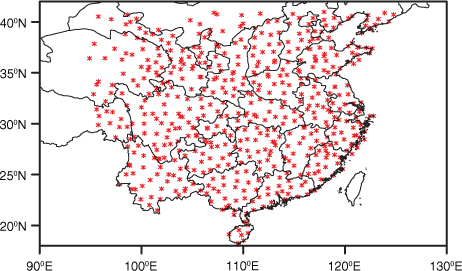
Fig. 1
The 565 observational stations used in this study.
The background fields used in our experiments are prepared very similarly with the ‘true’ case but they are produced from a 24-hour forecast initialised by the NCEP/FNL data at 24 hours prior to the analysis time. A sizeable difference is thus found between the ‘true’ state and the background fields. From the background fields at the analysis time, a 30-hour integration regarded as the control run (referred to as ‘CTL’) is obtained through the assimilation window to produce the basic states for assimilation and evaluate the results from both NLS-4DVar and POD-4DVar assimilation experiments.
A 4D moving sampling strategy (Wang et al., 2010; Tian et al., 2014) is adopted to produce the MPs (P x) and their corresponding simulated OPs (P y) from 78-hour forecasts with one output per hour and the background simulations. The POD-transformed OP and MP matrixes also can easily be obtained. The two 78-hour forecasts are initialised with 1°×1° NCEP/FNL global analysis data, respectively, at 24 and 48 hours prior to the analysis time. Each 78-hour forecast includes 73 six-hour moving windows and the ensemble size is 146 (=73×2) as a result.
In the following experiments, the performance of the NLS-4DVar method is examined in comparison to the POD-4DVar method. To have a fair comparison, all the assimilation settings (including the assimilated variables, the analysis time, the assimilation window, the observations, the sampling strategy, the ensemble size and the localization Schur radii) are the same. It should be noted that, like most 4DEnVar methods, we have to determine the localisation Schur radii for NLS-4DVar either by experience or through sensitivity experiments since only a static correlation matrix (31) is used in the current algorithm, which will definitely bring some uncertainty. This phenomenon is indeed observed in our real data assimilation experiments (e.g. Zhang et al., 2014). To assess the overall performance of the NLS-4DVar method (marked as ‘NLS’), especially in contrast to the POD-4DVar method (marked as ‘POD’), we first compare the root mean square errors (RMSEs) of 30-hour forecast of accumulated rainfall (from 1~30 hours after the analysis time) with the ICs from the ‘NLS’, ‘POD’ and ‘CTL’, respectively. Figure 2 shows the RMSEs of 30-hour forecast of accumulated rainfall with the ICs from the assimilations, both ‘NLS’ and ‘POD’ produce smaller values than those from ‘CTL’, which indicates both ‘NLS’ and ‘POD’ can steadily improve the rainfall forecast over 30 hours. Meanwhile, Fig. 2 also indicates that NLS-4DVar outperforms POD-4DVar moderately, due to the iterative strategy adopted in NLS-4DVar. Additionally, sensitivity experiments show that the NLS-4DVar solution is already convergent only after two iterations (i.e. I max=2).
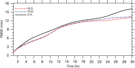
Fig. 2
RMSEs of 30-hour forecast of accumulated rainfall (from 1~30 hours) with the ICs from ‘CTL’ (solid line), ‘POD’ (long-dashed line) and ‘NLS’ (short-dashed line).
To further investigate the potential of NLS-4DVar, we also compare the difference of accumulated rainfall at 18 hours after the analysis time with the ICs from ‘NLS’, ‘POD’, ‘CTL’ and ‘truth’ in Fig. 3, respectively. Generally, ‘CTL’ and ‘POD’ share a stronger positive bias region around (26°~30°N, 122°~126°E). Correspondingly, NLS-4DVar only has a little weaker positive bias in the same region, which demonstrates the NLS-4DVar method can not only reduce the overall forecast errors but also ameliorate the detailed patterns of forecasted rainfall substantially. The results also suggest that NLS-4DVar works fairly effectively, as it does help to reduce the errors in both the immediate vicinity and outside of the observations even though the observational error is not negligible and the distribution of observations is sporadic and only at the land surface. Certainly, the superior performance of NLS-4DVar is attributed to its ability to provide a better description of the atmosphere and is closer to the ‘true’ state at the analysis by incorporating the observation information into the background. Figure 4 shows that the difference of temperature at the σ=0.512 level at the analysis time between ‘NLS’ and ‘truth’ is much smaller than those between the ‘CTL’, ‘POD’ and ‘truth’ as a whole. A significant decrease of the difference in the region (24°~41°N, 117°~128°E) appears in ‘NLS’ compared with ‘POD’ and ‘CTL’ (see Fig. 4a, b and c). Meanwhile, Fig. 4b and c also show that POD-4DVar can also improve the accuracy of the IC significantly, which leads to a general decrease (but less than NLS-4DVar) in the difference of temperature at the selected layer. Furthermore, to investigate the effectiveness of NLS-4DVar, we also compare the vertical profiles of RMSEs of some basic model variables from ‘NLS’ and ‘POD’ at the beginning and the end of the assimilation window, calculated at all horizontal model grid points of each layer. The same conclusion can be drawn that NLS-4DVar produces more accurate atmospheric states than POD-4DVar does. As seen in Figs. 5 and 6, NLS-4DVar yields a smaller error than POD-4DVar on most model layers. This implies that the iterative strategy adopted in NLS-4DVar really contributes to its superior performance.
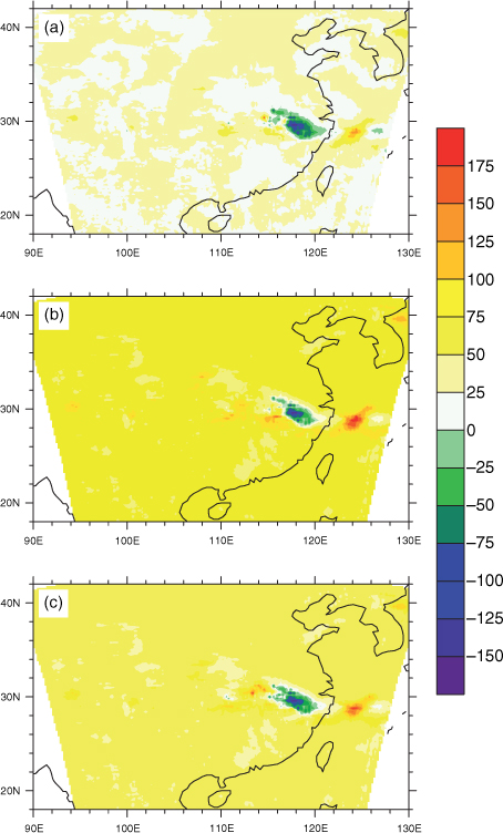
Fig. 3
Accumulated rainfall difference (mm) between (a) ‘NLS’, (b) ‘POD’, (c) ‘CTL’ and the ‘truth’ at 18 hours after the analysis time.
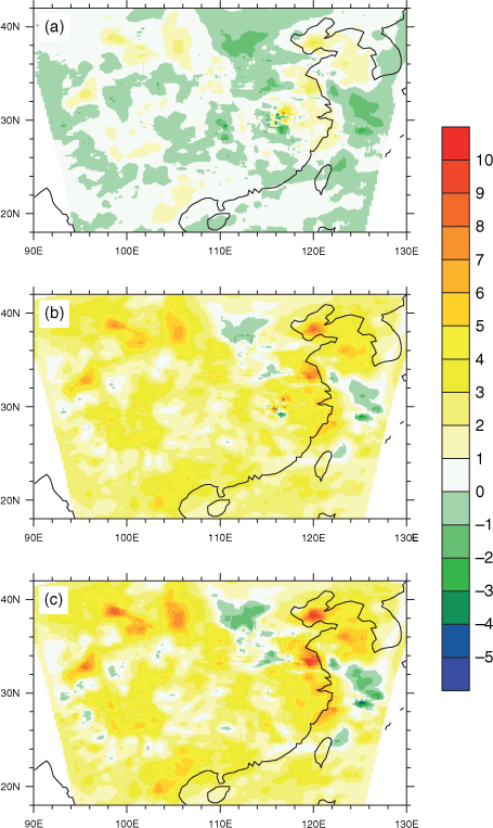
Fig. 4
Temperature difference (K) on the σ=0.512 level between (a) ‘NLS’, (b) ‘POD’, and (c) ‘CTL’ and the ‘true’ state at the analysis time.
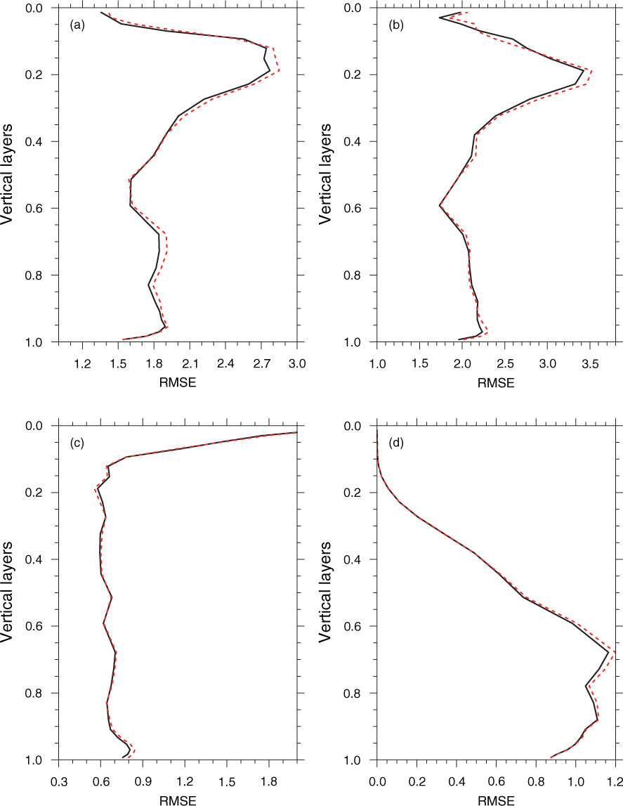
Fig. 5
Vertical profiles of RMSEs of (a) zonal wind (m s−1), (b) meridional wind (m s−1), (c) temperature (°C), and (d) water vapour mixing ratio (g kg−1) of ‘NLS’ (solid curve) and ‘POD’ (dashed line) at the start of the assimilation window.
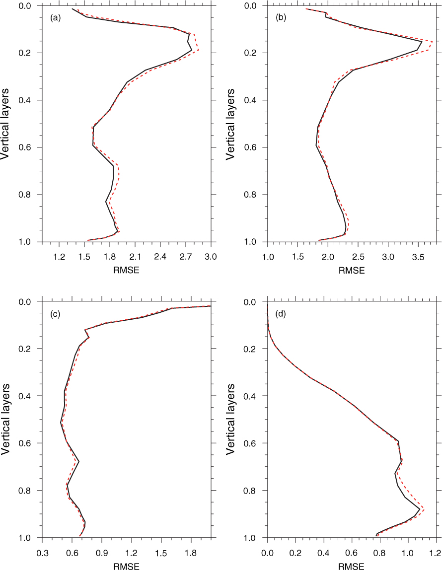
Fig. 6
Same as Fig. 5, but for at the end of the assimilation window.
4. Summary and concluding remarks
The existing 4DEnVar methods (e.g. Tian et al., 2008, 2011) are commonly based on the linear assumption between the MPs and OPs as their theoretical foundation. When the forecast model or observation operator is highly non-linear (frequently occurring in the actual assimilation implementations), the above linear assumption becomes problematic. As a result, its theoretical foundation collapses. To address this issue, a non-linear least squares iterative algorithm is proposed to iteratively approximate the optimal non-linear 4DVar solution in a computationally acceptable way, which defines the NLS-4DVar approach. Particularly, the iterative algorithm can produce satisfactory results with a cost of a very few iterations (only three iterations are used in our OSSEs), consequently, it can be implemented more efficiently than the standard adjoint-based 4DVar (Wang et al., 2010).
The effectiveness, robustness and potential merits of the proposed NLS-4DVar method are demonstrated by several sets of OSSEs based on the platform of ARW using accumulated rainfall-observations. For comparison, the original POD-4DVar method is simultaneously used to carry out the same OSSEs under the same conditions. Our main conclusions are summarised as follows:
NLS-4DVar can be easily implemented as the original POD-4DVar method by utilizing an explicit iterative equation rather than resorting to any existing optimization algorithm;
The solution of the original POD-4DVar method is only the first iteration of the NLS-4DVar iterative method, which largely explains inferior performance of POD-4DVar.
A group of OSSEs in a nearly realistic framework demonstrates that the iterative strategy employed in NLS-4DVar is able to alleviate the non-linear problems arising from data assimilation, the resulting NLS-4DVar method not only can reduce the overall forecast errors but also can substantially ameliorate the detailed patterns of forecasted rainfall.
Applications of NLS-4DVar in the meso- and micro-scale systems are expected to be favourable because of their high non-linearities.
As an ensemble-based method, NLS-4DVar also needs a moderation function to filter out the spurious long range correlations but only adopts a non-adaptive correlation matrix (which is usually determined either by experience or through sensitivity experiments) in current formulation. Extra efforts need be made to explore a flow-adaptive moderation of spurious ensemble correlations and its use in NLS-4DVar.
5. Acknowledgements
This work was partially supported by the National High Technology Research and Development Program of China (Grant No. 2013AA122002), the Knowledge Innovation Program of the Chinese Academy of Sciences (Grant No. KZCX2-EW-QN207) and the Special Fund for Meteorological Scientific Research in Public Interest (GYHY201306045). The authors would also like to thank two anonymous reviewers for their valuable comments and suggestions that are helpful for improving the paper.